


The Sigma-MT Suite (includes Sigma-MT EA and the Sigma-MT Scanner) is available now for new VIP Cycle Analysts (founding members). Please contact me (on X or Substack chat) once you have joined or upgraded from standard membership to receive the software.
Prerequisites: the full single-chart course, parts one through five, or at minimum the quick start, spectrogram and detection guides. The scanner assumes you can read a rank, a wavelength and a phase because it is about to hand you dozens of them at once!
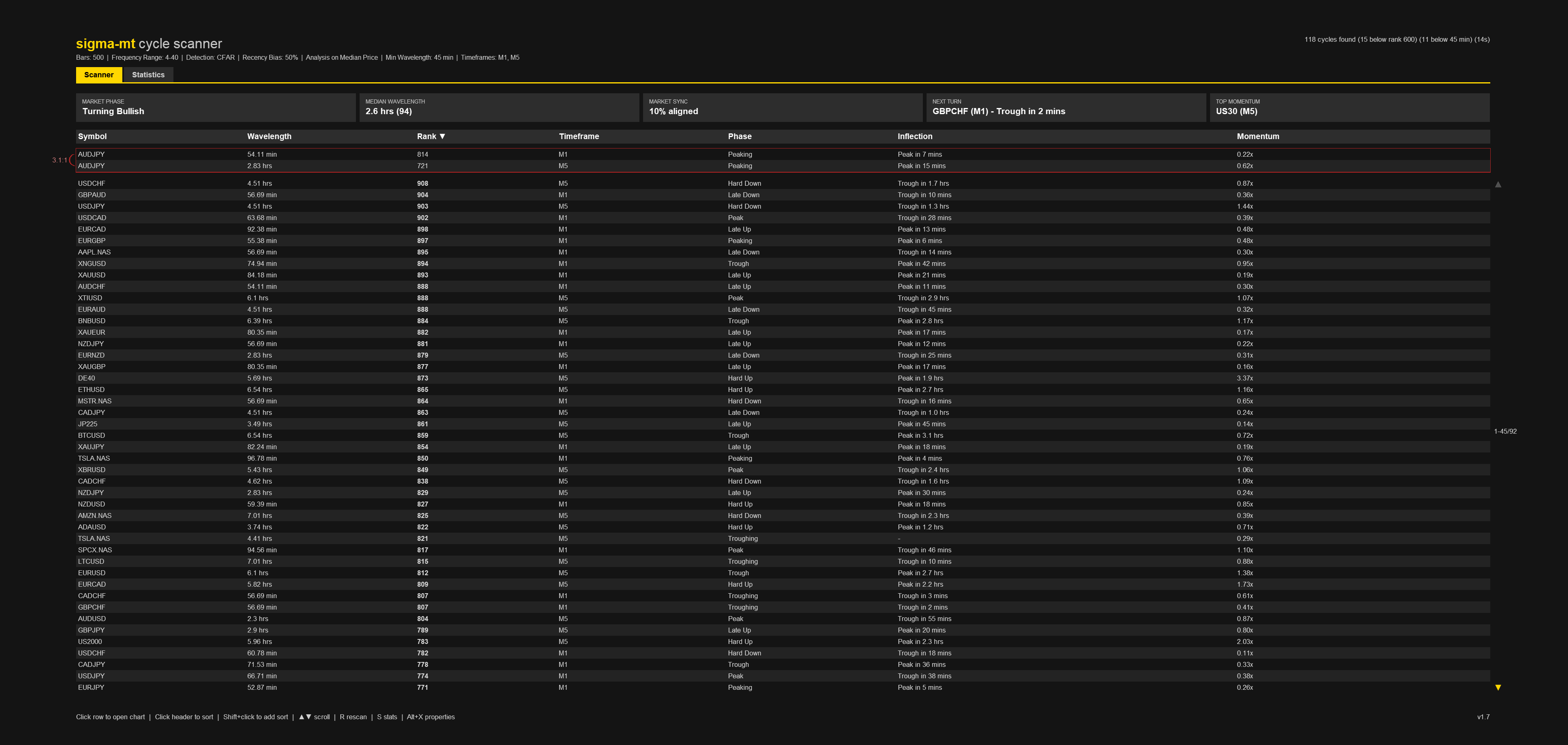
Everything this course has taught you so far is deliberate, single-chart work: attach the EA, read the spectrogram, judge the rank, project the turn. The obvious question follows you the whole way through. Which chart? A clean, high-ranking, well-phased cycle is a needle, and the market is a very large haystack; the trader who checks ten instruments by hand has still not checked the other two hundred. The Sigma-MT Scanner, (currently on version 1.7 and part of the Sigma-MT portfolio) exists to remove that problem entirely. It runs the same wavelet convolution, the same CFAR detection and the same quality scoring you know from the EA across every symbol in your Market Watch, on up to five timeframes at once, and returns a ranked, sortable table of every tradeable rhythm it finds. This part covers the operational half, getting it installed, configured and scanning. The next part covers reading what it returns and the part after that the click-through from scanner to chart for a full deep dive.
Install and the one-time template
The Scanner is itself an Expert Advisor. Copy it into MQL5\Experts alongside Sigma-MT, refresh the navigator, and attach it to any chart; the symbol and timeframe of that host chart are irrelevant, since the scanner ignores it’s host and takes over the window as a dedicated panel. Like the EA it places no trades and requests no permissions.
Before your first scan, do one piece of setup you will never have to repeat because it transforms the whole workflow later. Open any chart, attach Sigma-MT to it, configure the inputs however you like your analysis, then right-click the chart and save it as a template named SigmaMT, matching the Scanner’s SigmaMTTemplate input (in Chart Launch section), which defaults to exactly that name. Note, you can also use another name, if you wish just ensure they line up.
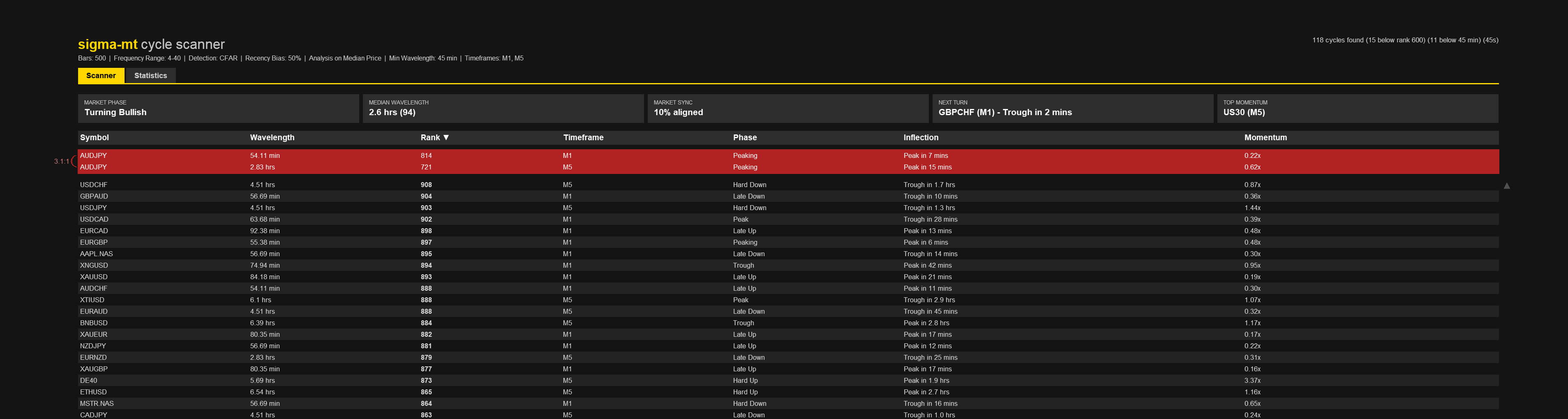
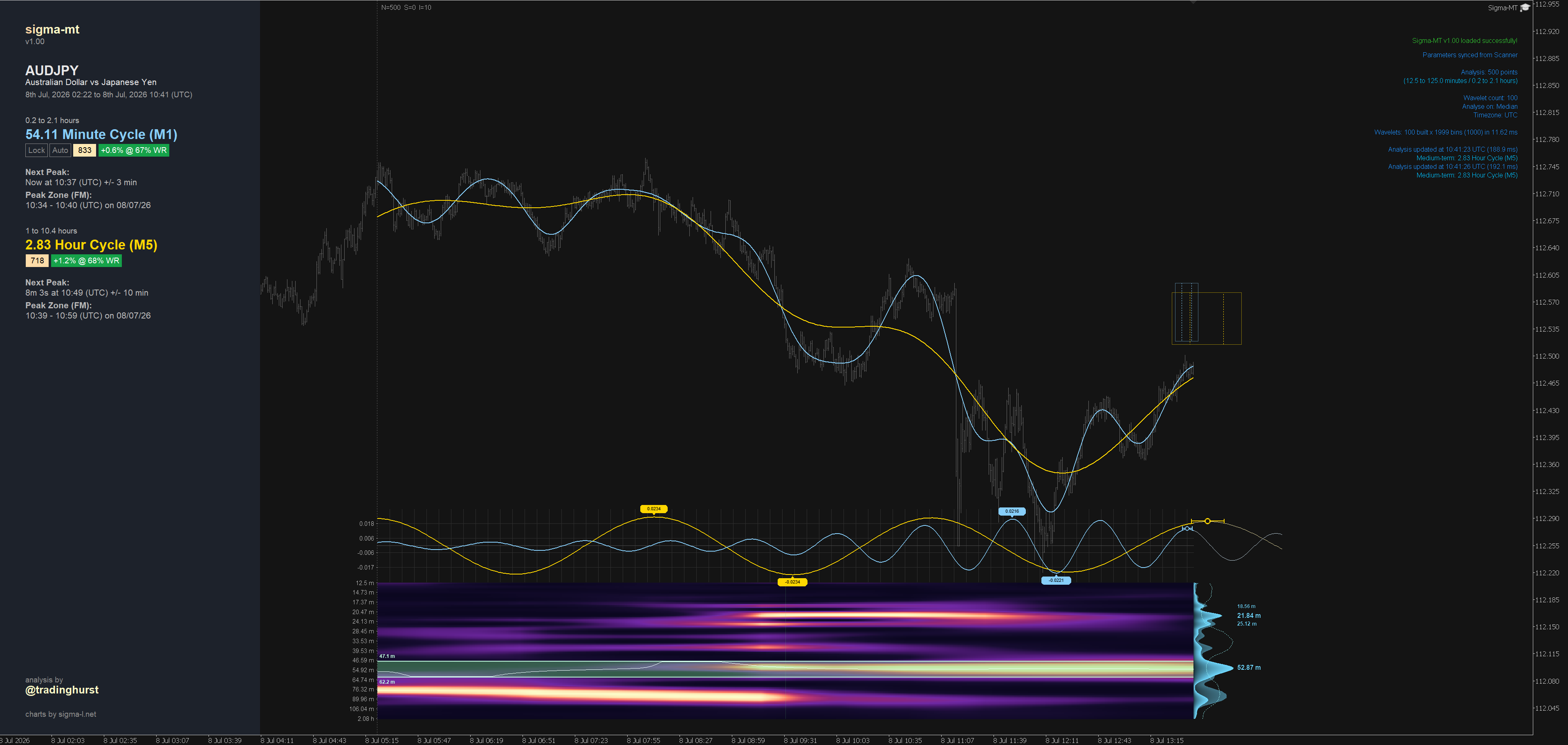
When you eventually click a result row, the scanner opens the suggested chart and applies this template automatically, so the cycle analysis appears pre-loaded with the EA rather than as a bare chart, matching the characteristics found via the scanner which uses the same engine. The parameter handoff that accompanies this is genuinely clever and gets full treatment in part eight; for now, just save the template and forget about it. If the template is missing the scanner will still open charts, with a warning in the log, and setting the input blank disables template application deliberately.
Choosing the universe
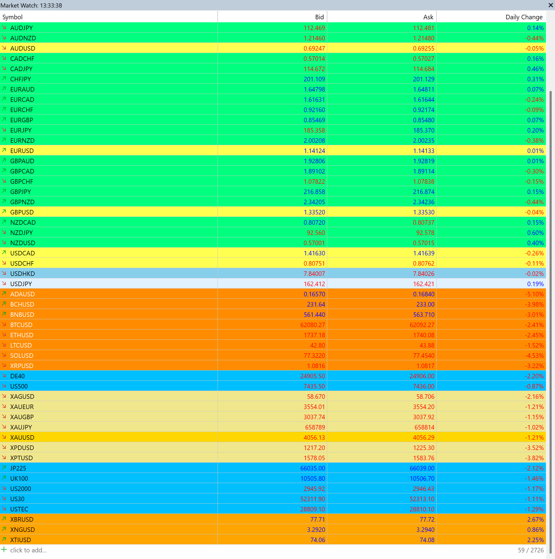
The Scanner’s universe is simply your Market Watch: every symbol currently shown there is scanned, and nothing else is. This is a deliberate design choice, because it means curating your scan list requires no configuration dialog at all, you add and remove symbols in the Market Watch exactly as you always have, and the next scan reflects it. Keep a lean, liquid watchlist and scans complete quickly; show hundreds of exotic crosses and the scan will dutifully churn through all of them. My own habit is a working set of the majors, the key crosses, the indices and the metals, which keeps a full multi-timeframe pass comfortably fast while covering everything I would realistically trade.
Timeframes and the analysis settings
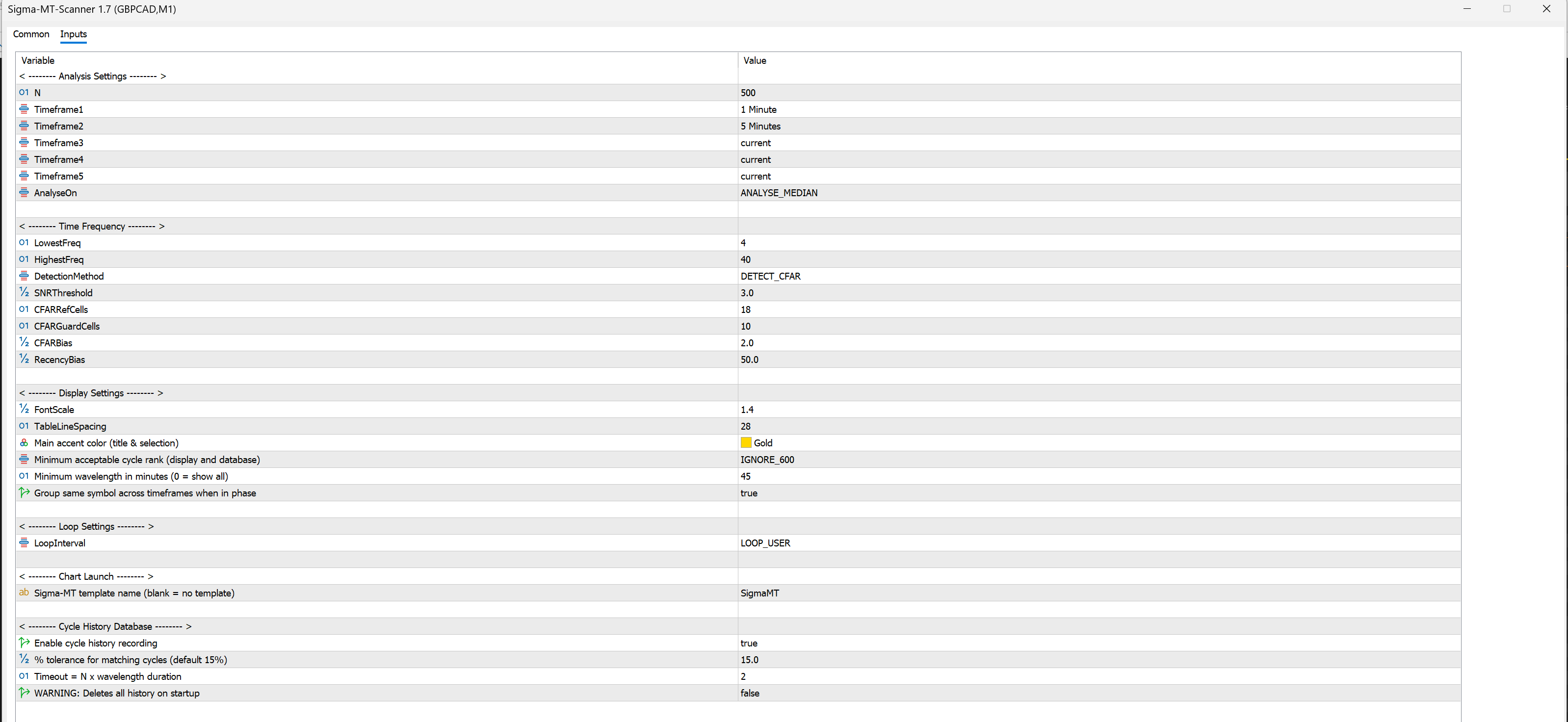
The Analysis Settings group offers up to five timeframe slots. Timeframe1 defaults to M1 and any slot left at current is disabled, so you enable exactly as many resolutions as you want swept, up to all five. Each symbol is analysed independently on each enabled timeframe, which is what later allows the Scanner to notice when one instrument is carrying related cycles at several resolutions at once, the nested-cycle grouping that part seven unpacks. Be aware the workload multiplies accordingly: five timeframes across a large watchlist is five full analyses per symbol, and the progress readout will show you the cost in time and processing accordingly. Scanning through my main market watch of around 60 instruments at N=500, across 5 timeframes, takes around 45 seconds! In practice one should aim for Market Watch lists around 30-50 instruments in order to avoid clutter if analysing multiple timeframes. I leave it up to the user to find their preferred balance of this powerful feature.
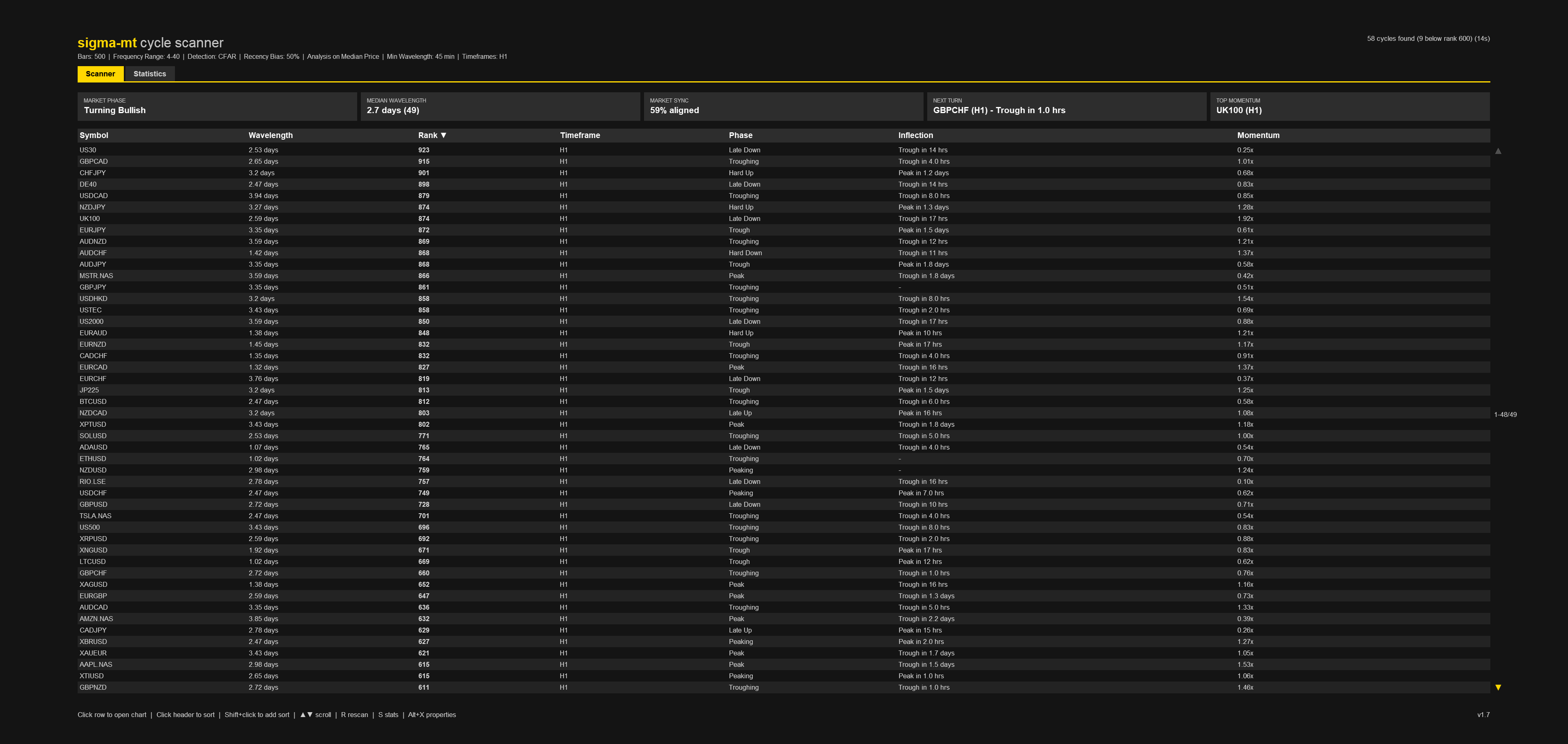
The rest of the analysis inputs you already know, because they are the same engine. N is the sample size per analysis, AnalyseOn the price it decomposes, and the Time Frequency group carries the identical LowestFreq, HighestFreq, DetectionMethod, SNRThreshold, CFAR cell and bias settings and RecencyBias from the EA, with the same defaults and the same meanings. This is worth a moment’s appreciation: the scanner is not a lightweight screener applying some crude proxy and hoping the EA later agrees. Every row in its results table earned its place through the full wavelet convolution and CFAR detection you studied in the detection guide, at the settings you chose. What the scanner calls rank is precisely the 0 to 1000 rank the EA shows you and so forth.
The three ways to scan
The LoopInterval input sets the scanning rhythm, and there are three modes of operation within it. Manual, the default, scans once when you press R and then waits for you; this is the mode I recommend while learning and for the session trader who wants a fresh sweep at moments of their choosing. Continuous begins a new scan the moment the previous one completes, keeping the table as live as your hardware allows, which suits a dedicated scanning terminal left running. Between the two sit the fixed intervals, one, five, fifteen, thirty or sixty minutes, where the Scanner rests between sweeps and refreshes on schedule; these are the sensible default for most people, frequent enough that the table stays current, quiet enough that your terminal is not permanently occupied. Whichever mode is set, R always triggers a scan on demand provided one is not already running, and the panel’s status line shows progress through the symbol list as it works.

Filtering the flood
A broad watchlist on several timeframes can return more rows than any human should triage raw, so the scanner filters at the source. IgnoreBelow sets the minimum acceptable rank for a cycle to appear at all, in tiers of 600, 700, 800 or 900, and I would encourage you to use it aggressively: the whole discipline of this course has been that detections below 700 deserve suspicion, and a scan-level floor simply enforces that discipline before the noise ever reaches your eyes. MinWavelengthMinutes discards cycles shorter than a chosen wavelength, expressed in minutes, which matters because a market-wide sweep of low timeframes will always find an abundance of very fast, technically valid but practically untradeable rhythms. A floor of an hour or two clears them out at a stroke. Set to zero it shows everything. Personally, if trading intraday, I set the minimum at 45 minutes - in my experience there is often great cycle features around an hour intraday but anything shorter is dicing with randomness just too much!

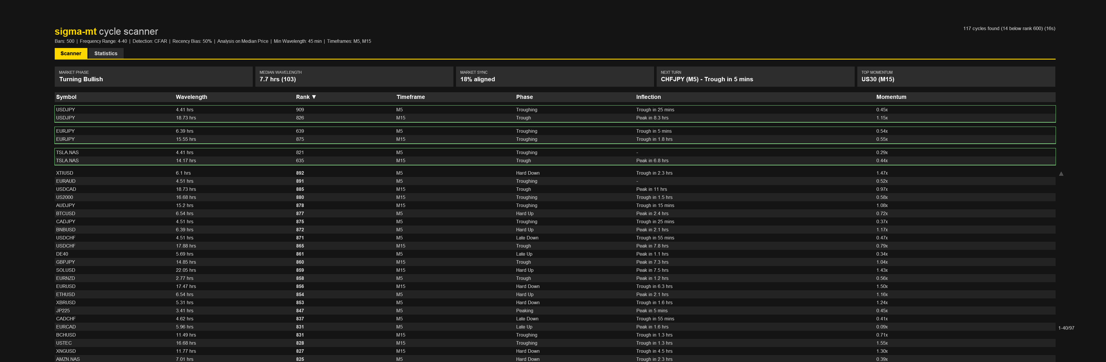
GroupInPhase, gathers rows of the same symbol across timeframes when their cycles are in phase, and it sits right on the border between operating the scanner and interpreting it. I will introduce it here and do it justice in part seven, where phase confluence and the harmonic validation behind that grouping are the entire subject.
Your first sweep
Put it together and the first session looks like this: Attach the scanner, confirm your Market Watch holds the instruments you actually care about, enable two or three timeframes to start, set IgnoreBelow to 700 and let it cook. Watch the progress line walk the symbol list, and when the table settles, simply read it with the eyes this course has given you: wavelengths in real units, ranks you know how to weigh, phases you know how to interpret. Click a column header to sort, shift-click to add a second sort, and scroll with the arrow keys. Press R to rerun the scan at a time of your choosing or set it to loop autonomously with the loop input described above.
Resist clicking through to charts for now; the next part is about extracting the full meaning of this table, the phase confluence between it’s rows and the harmonic relationships that mark a genuinely special result. The process after that completes the journey from a row in the table to a fully audited trade candidate.
Where to go next
Part seven, Reading the Results: Phase Confluence and Harmonic Validation, takes the table you can now produce and teaches you to read it the way the engine intends. What each column asserts, why in-phase cycles across timeframes are grouped together and the harmonic test that separates coincidence from genuine nested structure.