


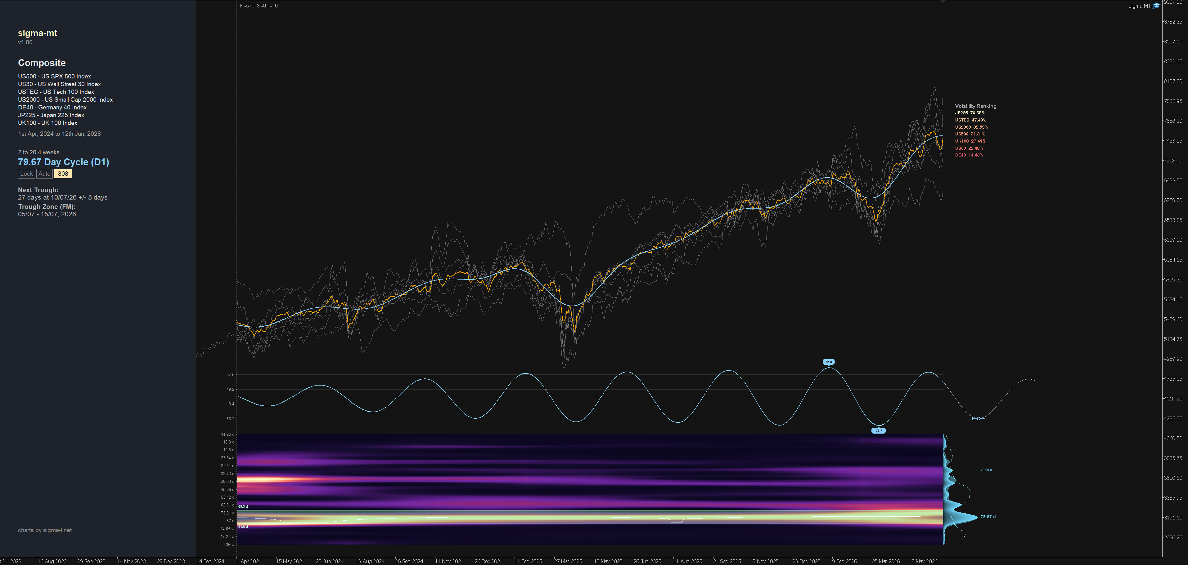
What is Sigma-MT?
Sigma-MT is an advanced Expert Advisor for the trading platform Meta Trader 5, available exclusively to VIP cycle analyst members on Sigma-L (founding members).
It is a direct port and enhancement of the python/numpy version I have developed over the last few years and has been seen previously in posts on Sigma-L. It is a bespoke, unique and powerful way to detect, analyse and act upon statistically significant periodic features in financial markets. It abstracts away many of the more technical aspects of this approach but retains a great degree of adaptability, alongside a streamlined interface and fast computation (processor dependent!). I hope you will enjoy using it as much as I do and discover some cyclic gems in the process.
Sigma-MT is not an indicator/expert advisor in the usual Meta Trader sense. It is a time-frequency analysis engine, drawn from the same family of mathematics used in radar and seismology, pointed at price. Rather than smoothing price and hoping a crossover means something, it decomposes the series into it’s component frequencies, watches how their power evolves through time, and tells you which cycle is dominant right now, where that cycle sits in it’s phase, and how much confidence the detection deserves.
This guide takes you from a fresh install to reading that information. Everything deeper, from the detection mathematics through projection, yield statistics, composites and the Sigma-MT Scanner has its own guide in this series. Here we simply get you on the chart.
For a complete reference to all of the controls for analysis navigation, see Sigma-MT keyboard reference.
For a complete reference to all in the input parameters, see Sigma-MT v1.0 Input Reference
1. Install
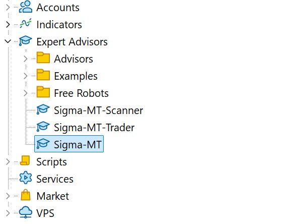
Copy Sigma-MT.ex5 into your MT5 data folder under MQL5\Experts (in MT5, go to File → Open Data Folder), then restart the terminal or right-click Expert Advisors in the Navigator and hit Refresh.
Sigma-MT places no trades. It is pure analysis, so there is nothing to configure on the trading side: no DLLs, no web requests, and no permissions beyond a standard EA attach.
2. Attach to a chart
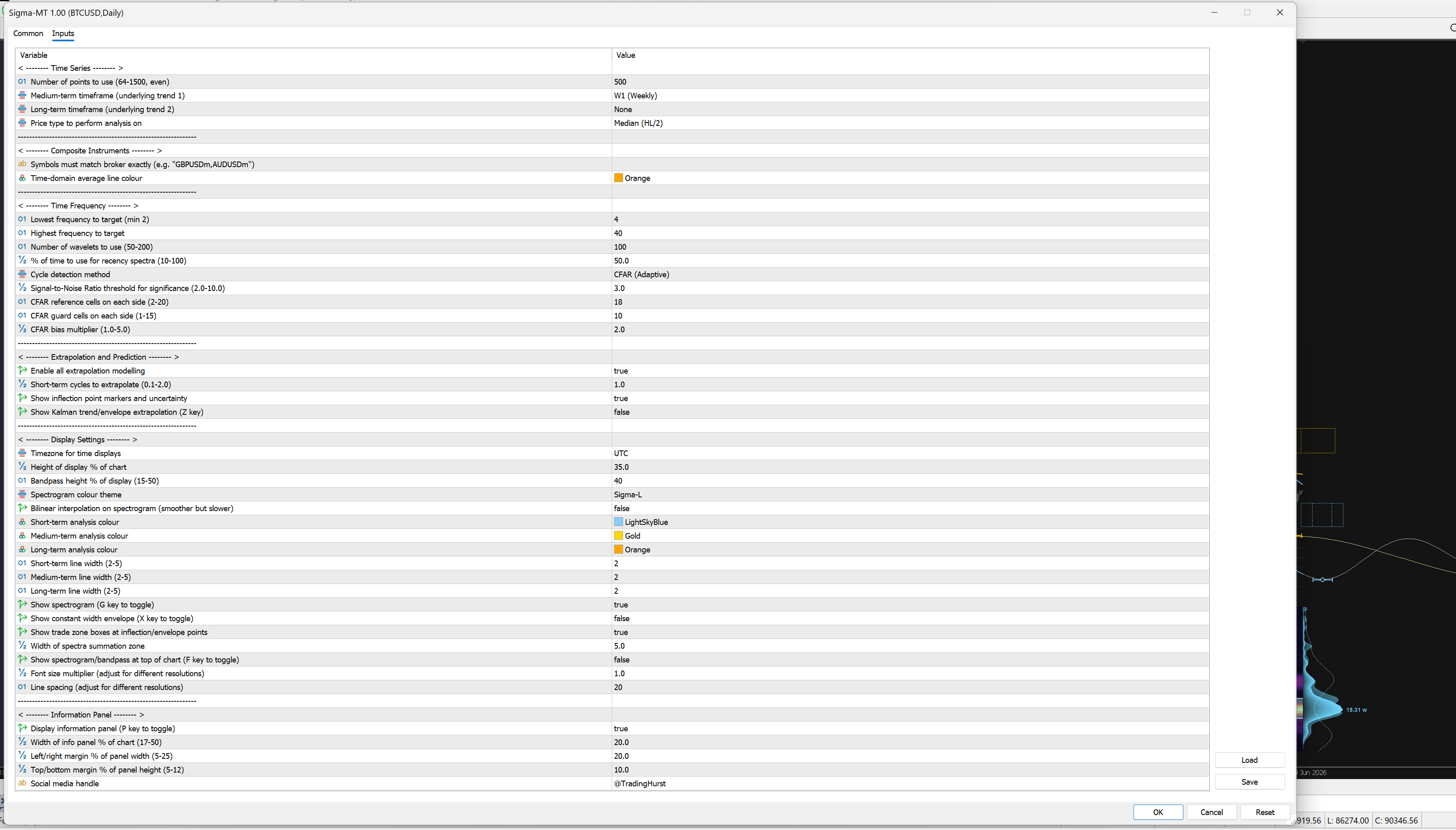
Open a chart on anything liquid. A major FX pair or an index on H1 makes a good first run. Drag Sigma-MT onto it and the input dialog will appear. For your first analysis, change nothing. The defaults are the configuration I run daily: CFAR detection, a target range of 4 to 40 cycles across the sample window, trade boxes on, and the info panel on. Click OK.
One constraint is worth knowing up front. Sigma-MT pauses on the monthly timeframe, because there simply are not enough MN1 bars to support meaningful spectral analysis. Weekly and below is it’s territory.
Within a few seconds the engine completes its first wavelet convolution pass and the display builds at the bottom of the chart.
One aspect worth adjusting at the outset is the display resolution of the panels. This can be adjusted in several ways in the ‘Display Settings’ and ‘Information Panel’ settings. Play around with font sizes and width/height adjustments to fit your screen size as appropriate. Save as an EA preset or save the whole chart as a template named ‘default’ to automatically load this setup on every chart that is launched (not recommended!). Alternatively save as a named template, such as ‘SigmaMT’ so you can load in the settings quickly if required on future charts. This will also be needed when we come to setup the Sigma-MT Scanner workflow.
3. What you’re looking at
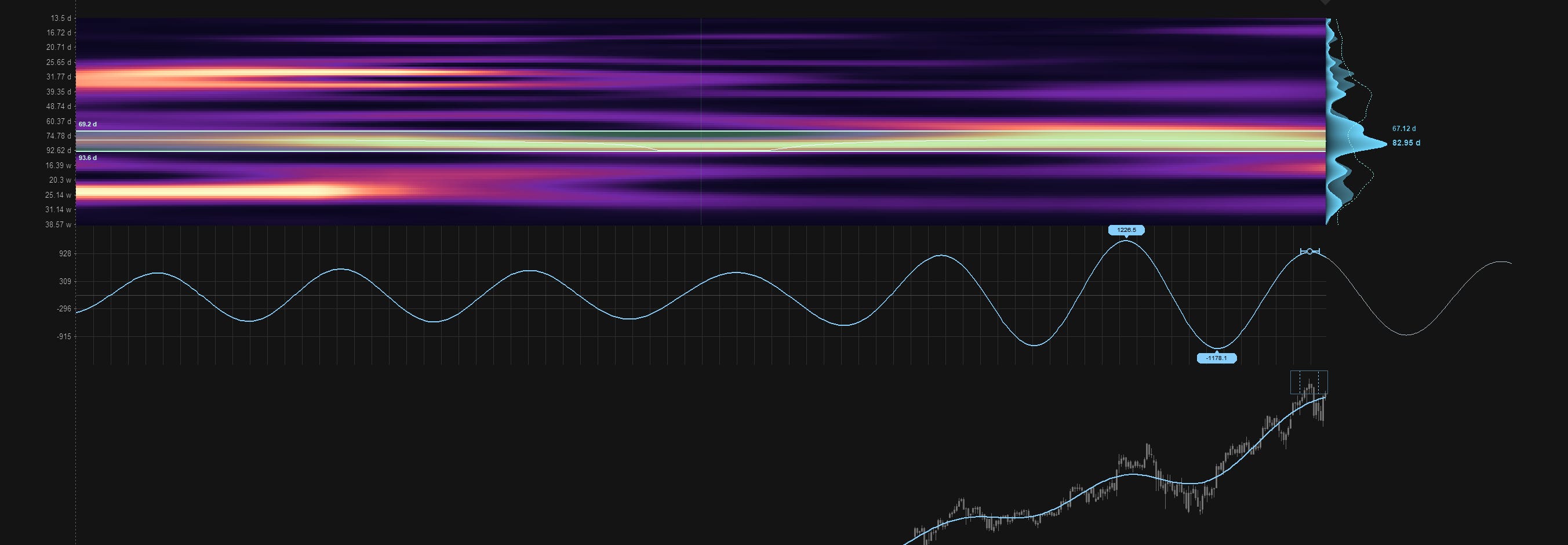
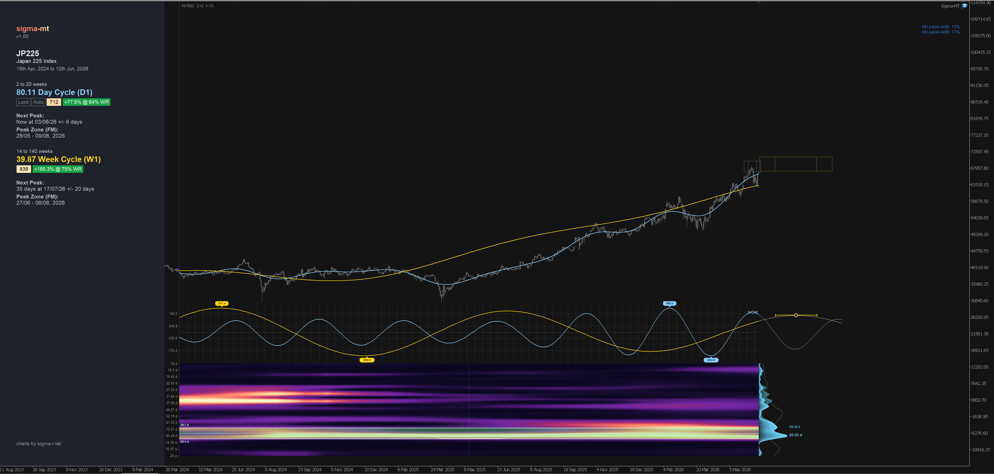
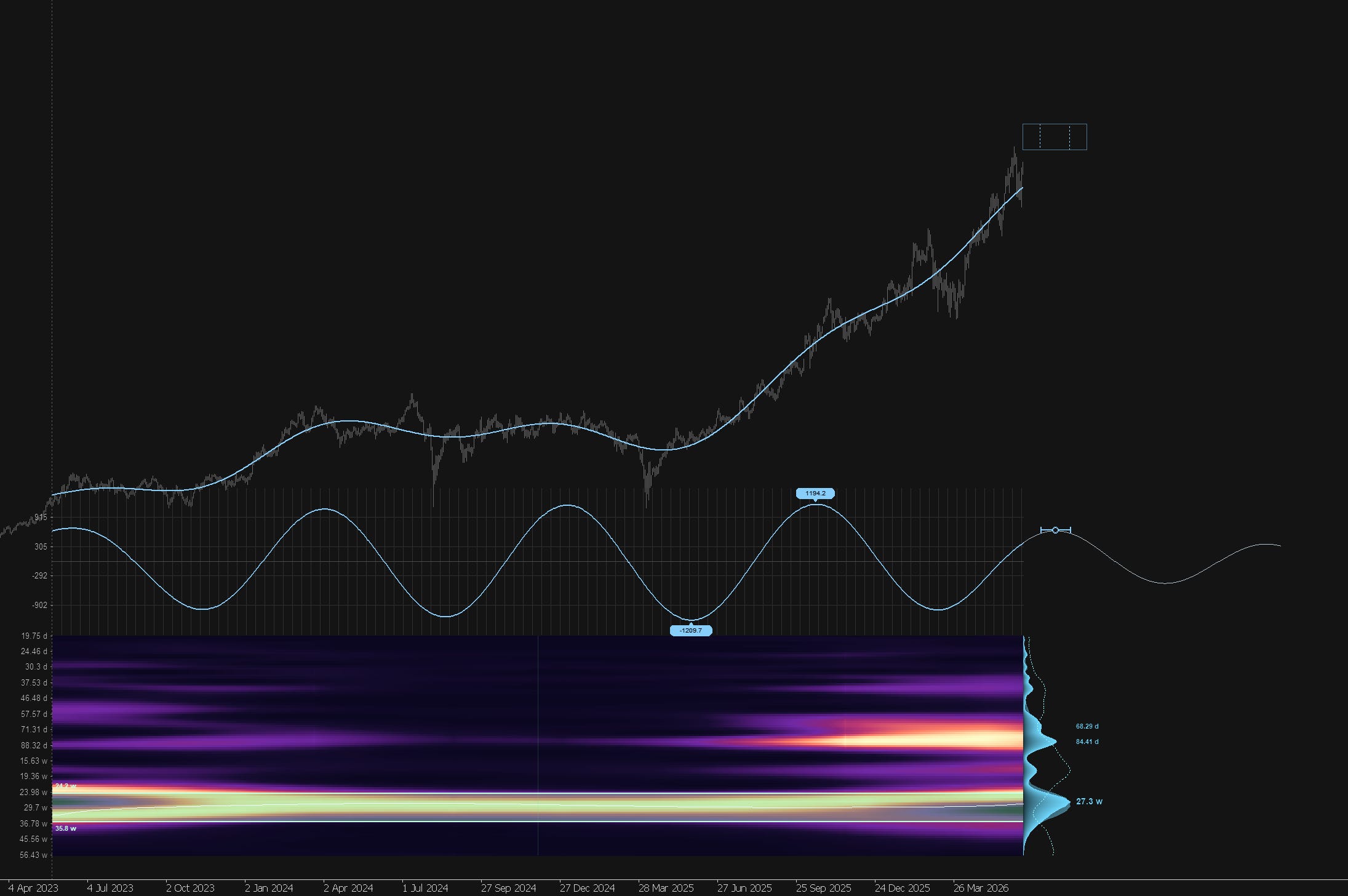
Three things appear, and together they carry the entire read. The spectrogram is the heart of the system. Time runs left to right, cycle wavelength runs bottom to top, and colour intensity shows spectral power. A bright horizontal band is a cycle that has persisted (it is stationary), and that persistence, rather than any single point, is what makes a cycle worth your attention for possible trading. To the right of the spectrogram, the summed spectrum shows where power concentrates across frequencies, with the detection threshold overlaid so you can see exactly what the engine considers significant.

Above/below it sits the bandpass panel (press F if you prefer it at the top of the chart). This is the dominant cycle extracted from the noise and plotted as a clean oscillation, with its projection extending past the current bar. It is the Hurst idea made explicit: isolate the dominant rhythm, then let its phase tell you where you are in the swing.
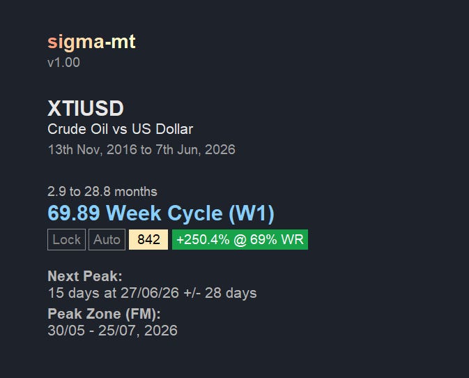
On the left you have the info panel, which summarises everything into a glance. It shows the detected wavelength in real units such as hours or days, the current phase status indicating whether the cycle is at a trough, rising, peaking or falling, and a score box grading detection quality from 0 to 1000 (1000 being a perfectly stationary sine wave and impossible in real markets!) over the recent window. Treat that score as your gatekeeper. Anything above 650 is worth attention, 800 and up is a solid detection, and 900 or more means the engine has found an unusually clean cycle. Below those levels, stand aside, and remember that the absence of a detection is also information.
4. Your first interactions
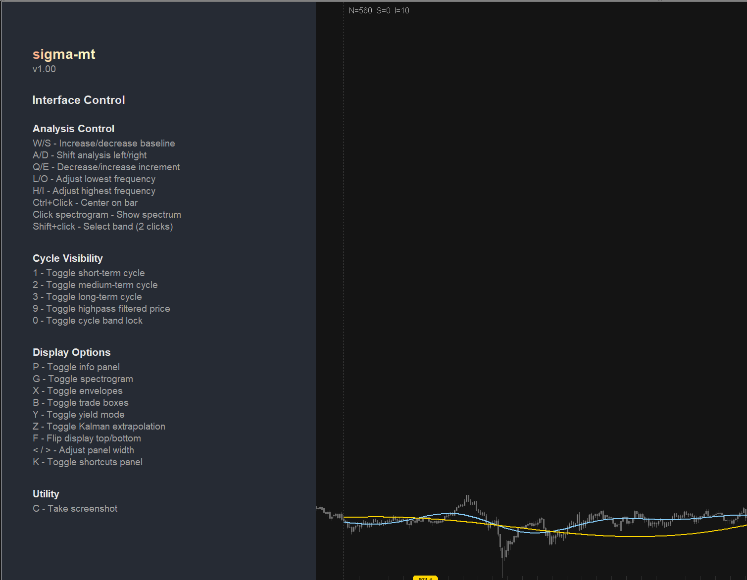
Press K and a shortcuts panel opens listing every keyboard control, grouped by function: analysis, cycle visibility, display options and utilities. You do not need to memorise anything, because K is always there. Press it again to close.
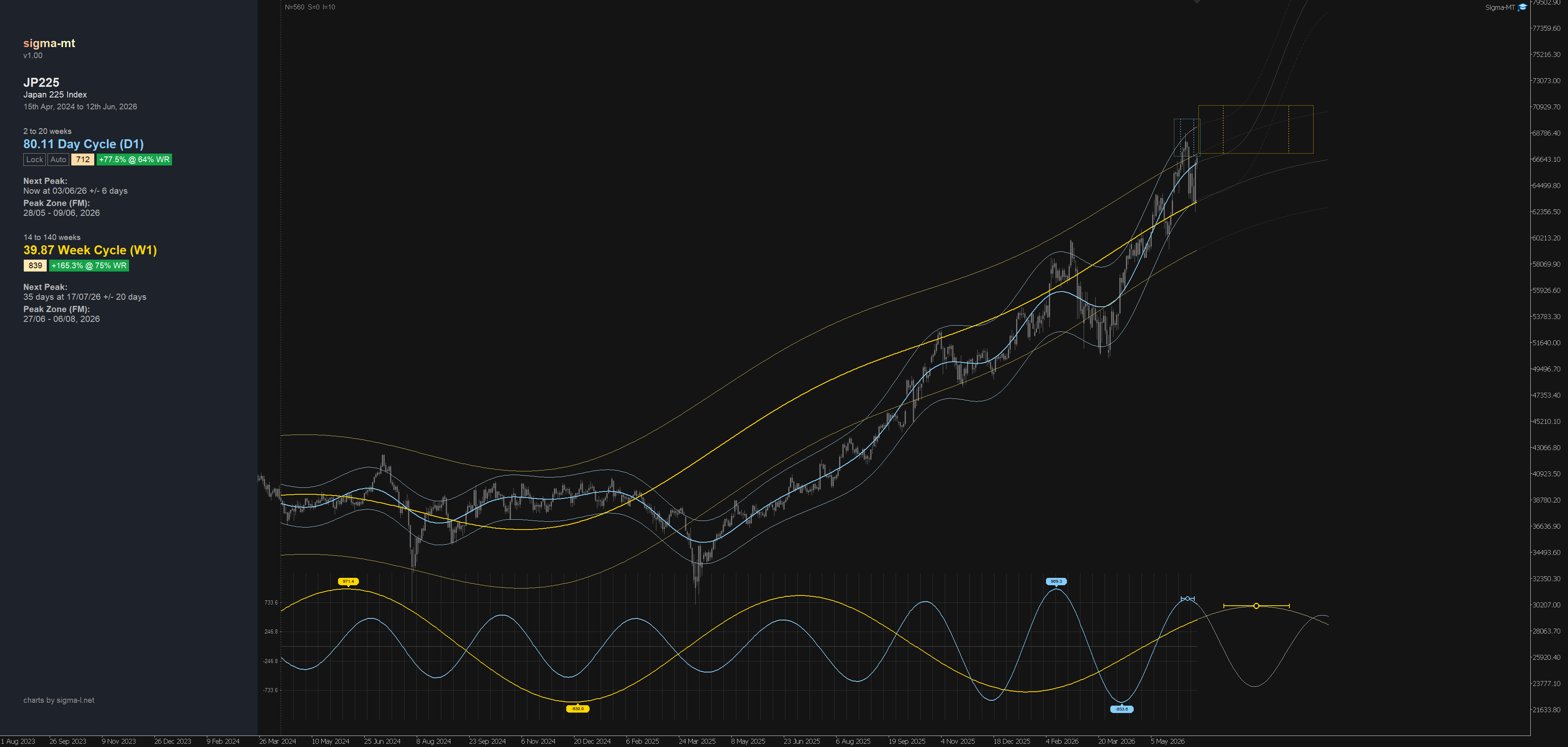
Now try the controls you will use constantly. The number keys 1, 2 and 3 toggle the short, medium and long-term cycle overlays (the medium and long-term layers activate once you enable their timeframes in the inputs, which Guide 2 covers properly). Press X to draw constant-width envelopes around price, calibrated so that price respects them roughly 95% of the time. Press B to toggle the trade boxes that mark projected inflection zones, and Z to switch on the Kalman extrapolation of the underlying trend. If you want a clean chart, G hides the spectrogram, and C captures a screenshot straight to disk.
There is one mouse interaction worth learning immediately. Click anywhere on the spectrogram and the summation area shows you the frequency spectrum at that exact point in time; click outside it and the view returns to the summed spectrum. Scrubbing through spectral history this way will teach you more about how cycles emerge and decay than any paragraph I can write.
5. Shaping the analysis window
Everything Sigma-MT tells you is computed over a window of bars, and that window is entirely under your control from the keyboard. Press W to extend the sample size and S to contract it. The current size is always visible in the small label beside the dotted line marking the start of the analysis, shown as N= along with S= for the shift and I= for the increment. The engine accepts anything from 64 bars up to 1500, and it will keep the count even for you automatically, since the wavelet transform requires it.
Why would you change it? Because the window defines what the engine can see. A short window resolves recent behaviour sharply but cannot detect a cycle longer than the data it holds, while a long window reveals the slow rhythms at the cost of diluting recent changes. If the spectrogram shows strong power pressed against its upper edge, that is usually a cycle bigger than your window, and a few presses of W will bring it fully into view. The frequency targets are defined per window, so resizing also rescales what each row of the spectrogram represents in real time units; the info panel always translates the detected wavelength back into hours or days for you.
Each press moves the size by the current increment, which you control with Q to halve it and E to double it, anywhere from 1 bar up to 100. Set a coarse increment to reposition quickly, then drop it down for fine adjustment. The I= value in the start line label always shows where it stands.
Shifting through history
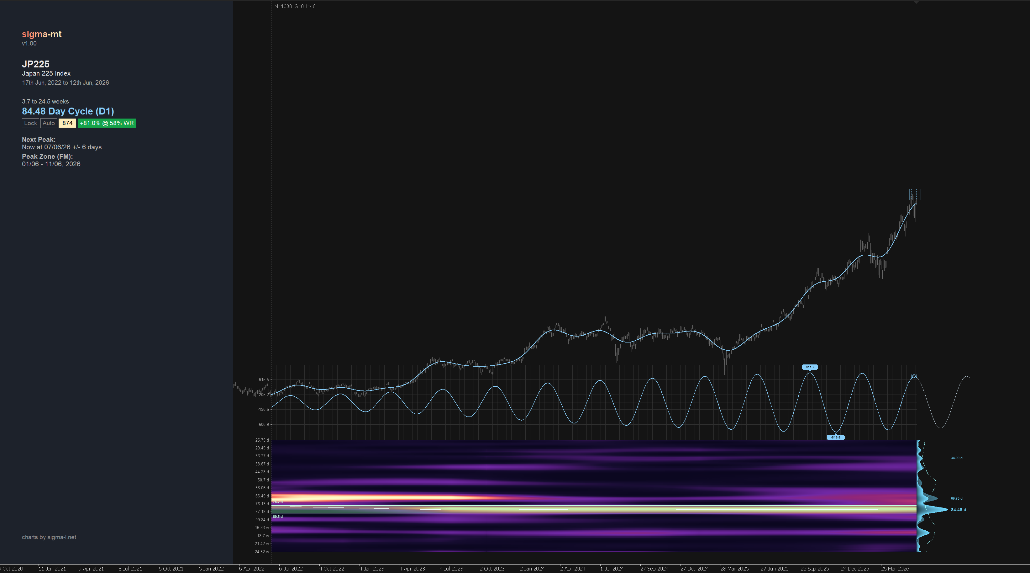
The window does not have to end at the current bar. Press A to slide the entire analysis into the past and D to bring it back towards the present, again moving by the increment each press. The S= value shows how many bars into history you currently sit, and when it returns to zero the engine confirms you are back at the live edge. The only limits are the data itself, since the EA will stop you when there is no longer enough history to fill the window, and one display restriction: the price envelopes are unavailable while shifted into the past, because their calibration only has meaning at the live edge.
This is one of the most instructive things you can do with the software. Park the window over a past period, look at what the engine detected and projected with only the data available at that moment, then step forward with D and watch how the cycle evolved. It is the closest thing to a flight simulator for cycle analysis, and it costs nothing.
For larger jumps there is a faster route than holding D. Hold Ctrl and click anywhere on the price chart and the analysis window recentres on that bar, placing it at the middle of the sample. One click takes you from the present to a period of interest months back, and another Ctrl+Click near the right edge, or a few presses of D, returns you home.
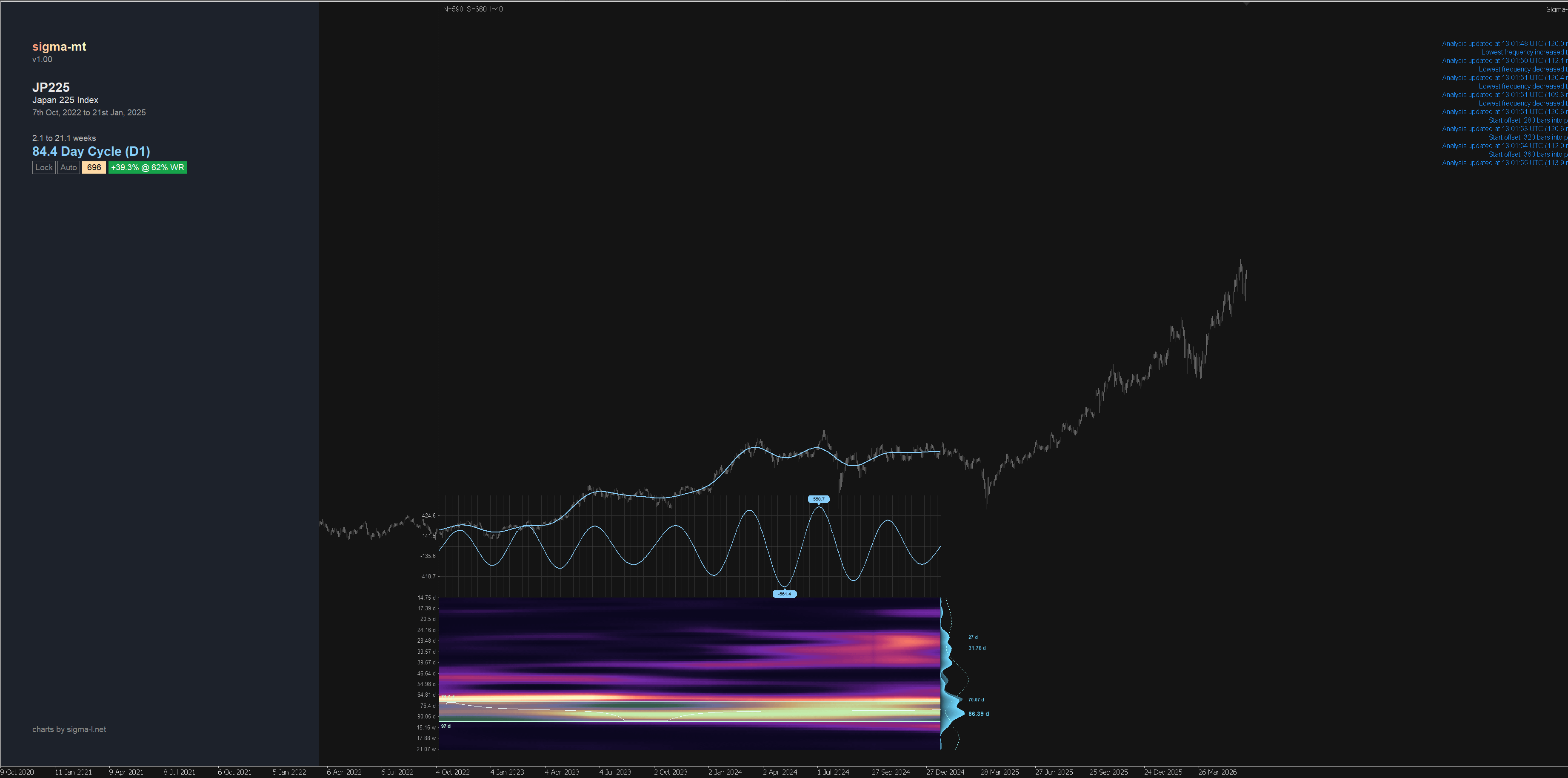
Moving through the spectrogram with HILO keys!
The vertical extent of the spectrogram is set by the lowest and highest frequencies the engine targets, and four keys let you reshape that band live. L and O move the low-frequency edge, which governs the longest wavelengths at the top of the spectrogram: L pushes it down towards 2, admitting longer cycles, while O raises it towards 10, trimming them away. H and I move the high-frequency edge at the bottom: H lowers it towards 15, cutting out the fastest, noisiest wavelengths, and I restores them up to the maximum of 40.
In practice these keys are how you walk up and down the frequency axis. If the action you care about lives in the slower cycles, press H a few times to discard the high-frequency clutter and the engine re-spreads its full wavelet budget across the band that remains, so resolution improves exactly where you want it. If a fast intraday rhythm is your target, push the low edge up with O instead. Every adjustment triggers a full re-analysis, and the detection, score and projection all update against the new band, so you can watch in real time how the dominant cycle call depends on where you point the engine.
A useful habit: when a detection seems ambiguous, nudge the band edges and see whether the call survives. A robust cycle keeps being found as the band shifts around it. A fragile one vanishes the moment its supporting noise is excluded, and that fragility is exactly what you want to discover before committing to the projection.
Selecting a custom band
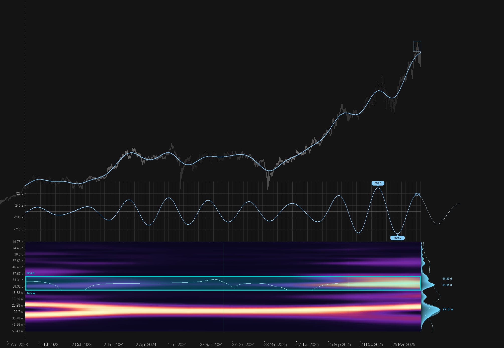
A very useful aspect of the app is the ability to select a custom band of 2 or more frequencies (wavelengths) to examine from the spectra. Simply shift+click once on the spectra to draw one boundary of the band and whilst still holding shift, click somewhere else in the band to establish the bandwidth and second boundary. The panel will also indicate this is a custom (not automatically detected) band, selected by the user.
Press the ‘0’ (zero) key to return to auto detection and remove the custom band of selected wavelengths.

6. Read the cycle
Here is the whole workflow in miniature. First check the score and ask whether the detection deserves your trust. Then check the wavelength and ask whether this is a rhythm you can actually trade on your timeframe. Finally check the phase. A cycle at its trough and rising argues for longs into the projected peak, while a cycle peaking and rolling over argues the reverse. The trade boxes translate that phase logic into a zone on the chart where the next inflection is expected, drawn with an honest uncertainty window rather than a single line of false precision.
That is a complete first analysis, and you have touched perhaps a few keys to help you get around. What you have not yet done is understand why the detection fired, or how to audit a cycle’s historical performance with yield mode on the Y key. That is deliberate. Each of those topics earns its own guide.
Where to go next
Guide 1, Reading the Spectrogram and the Time-Frequency Engine, is the natural next step. It explains what the engine is actually computing and how the short, medium and long-term layers stack into a genuine multi-timeframe read. From there the course runs through detection, projection, yield, composites and the market-wide Sigma-MT Scanner.