

The Moving Average - Band Pass Filter
The bandpass is the most powerful of the filter types we can exploit using the simple moving average. Learn how to design your own bandpass in this article

What is a Band Pass Filter?
In signal processing and the related topic of time-series filtering we often hear the terms ‘low pass filter’, ‘high-pass filter’, ‘band pass filter’ or ‘band stop filter’. They each refer to the process of creating a new signal with part of the original signal removed, or ‘filtered’. In the case of the high pass filter we remove the lower frequency components from a signal and retain the higher frequencies; we allow the higher frequencies to pass. This was achieved in the previous article with the help of a moving average - a particular type of low pass filter when plotted correctly to account for the digital filter lag. When the filtered (low passed) signal was subtracted from the original signal all that remained of the original signal were components above the cutoff (the span, or period) of the low pass filter. The resulting signal had therefore been highpassed. Highpass filters are useful to detrend time series or examine lower magnitude, higher frequency components of a signal.
We can take a similar approach to construct a bandpass filter. Instead of leaving one end of the frequency spectrum open as is the case for the low and high pass filters we can combine two low pass filters of different cutoffs (in the moving average case, periods or span). The distance between these two cutoffs is the passband of the filter. Any components with wavelengths in this passband will be passed by the filter and retained in the output signal.
A Recipe for Extraction
For the moving average bandpass filter recipe we will need three ingredients: a signal and two moving averages (low pass filters). The latter will form the bandpass filter. One of the moving averages should be set to a period lower than the other or vice versa. The exact specification of the moving average periods will vary depending on the signal component we wish to isolate and extract.
The bandpass filtered signal output is calculated by subtracting the lower frequency moving average from the higher frequency moving average.
It is paramount both moving averages are correctly lagged in time ( (odd period-1)/2) ) prior to the subtraction for the output to be accurate! The subsequent bandpass output is then plotted with a lag equal to the lower frequency moving average lag period.
As with most time series calculation it is often best to see the results visually. Below follows several examples of using this technique in action on a composite, simulated signal.
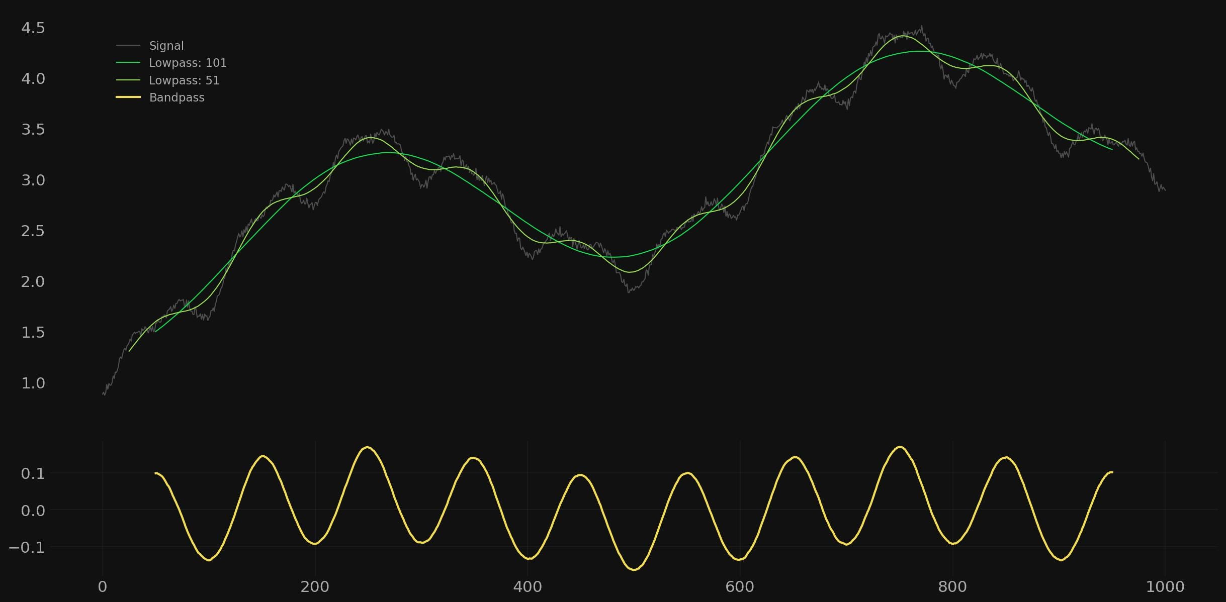
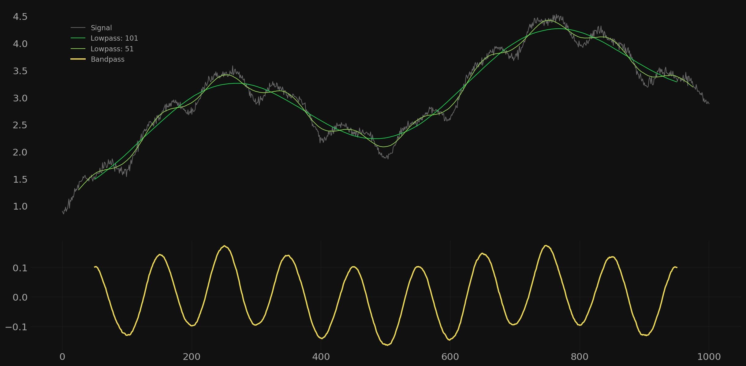
Example 1
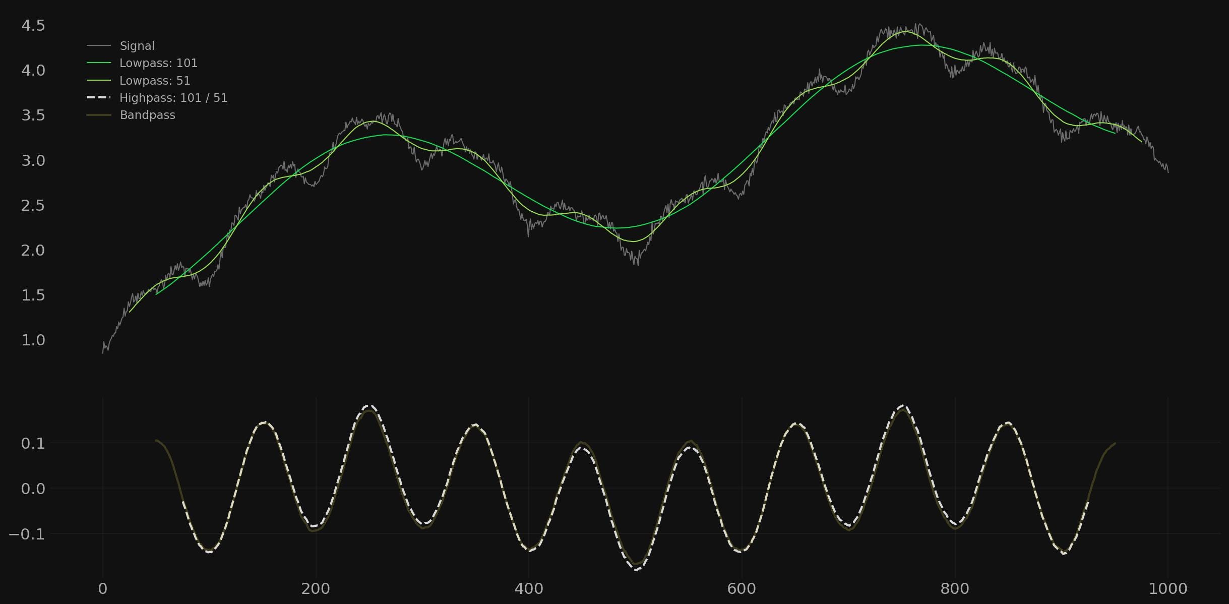
In this first example we have a signal of 1000 data points in length. The signal is a composite of white noise and sinusoidal components of wavelength: 500, 100 and 50, each of diminishing amplitude. A linear trend is also applied to the signal to simulate a smooth underlying motion.

In this first example we wish to isolate the component of 100 wavelength. Therefore we will set our low pass filters accordingly and construct two moving averages of period 101 and 51. The longer period moving average is set at the closest odd number available to attenuate the 100 wavelength component almost completely. Therefore when this signal is subtracted from the higher low pass filter the component of 100 will be retained. The higher frequency low pass filter is set around the closest odd number to the wavelength of the component at 50. Therefore the signal at a wavelength of 50 is almost completely attenuated and will not come through in the bandpass calculation.

We then perform the calculation to form the bandpass by subtracting the lower frequency moving average from the higher frequency moving average, leaving a band of data inbetween cleanly passed and retaining the signal of 100 wavelength. Importantly the bandpass is plotted so it is aligned with the lower frequency moving average lag.
The extracted bandpass signal has virtually no trace of high frequency noise and the higher frequency component at 50 is non-existent.
Example 2
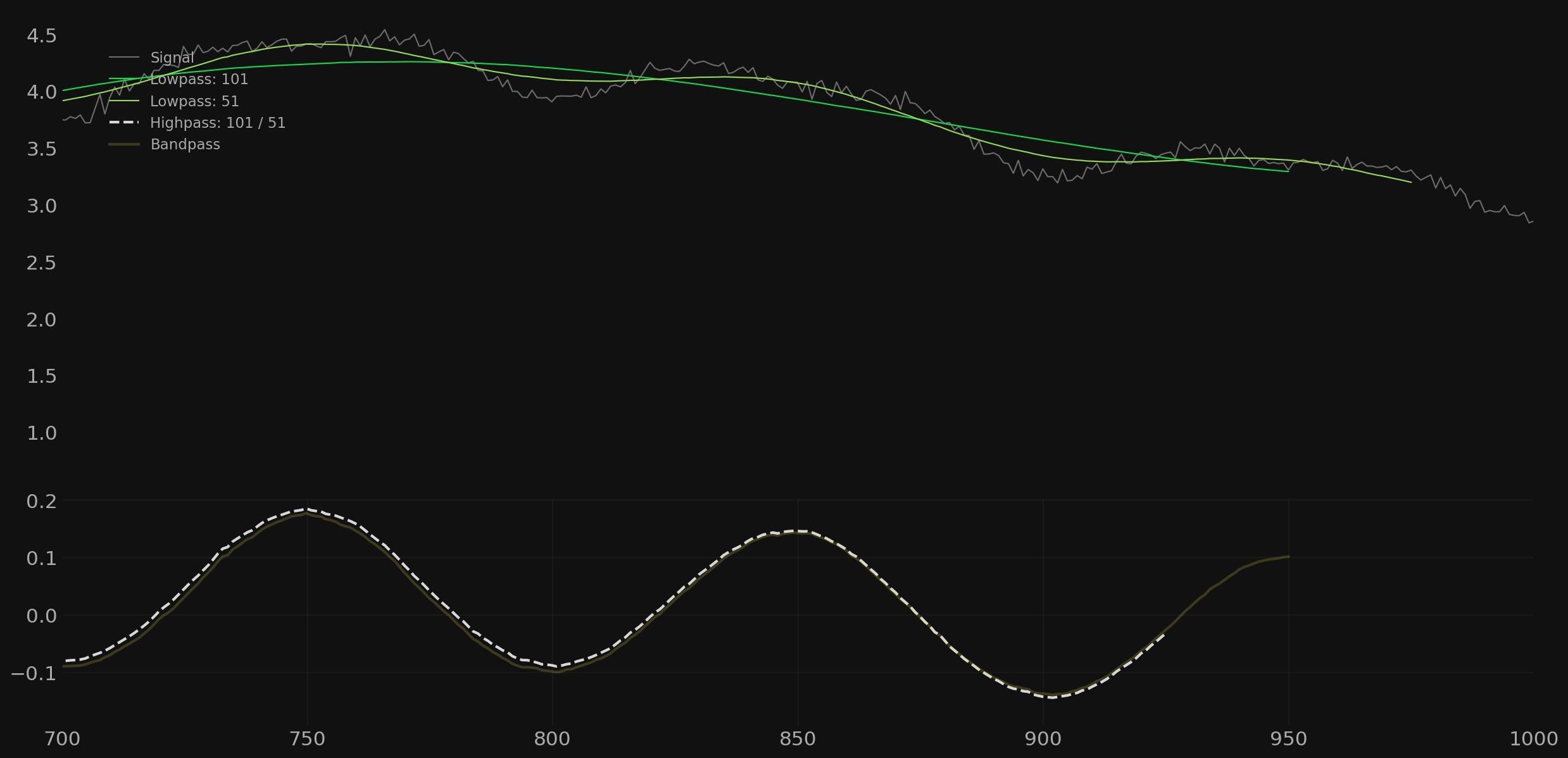
For the next example we will compare the outputs of the high pass filter and the bandpass filter. Below is the same signal with the bandpass filter applied as above and a highpass filter applied to retain all components of 100 wavelength and above.
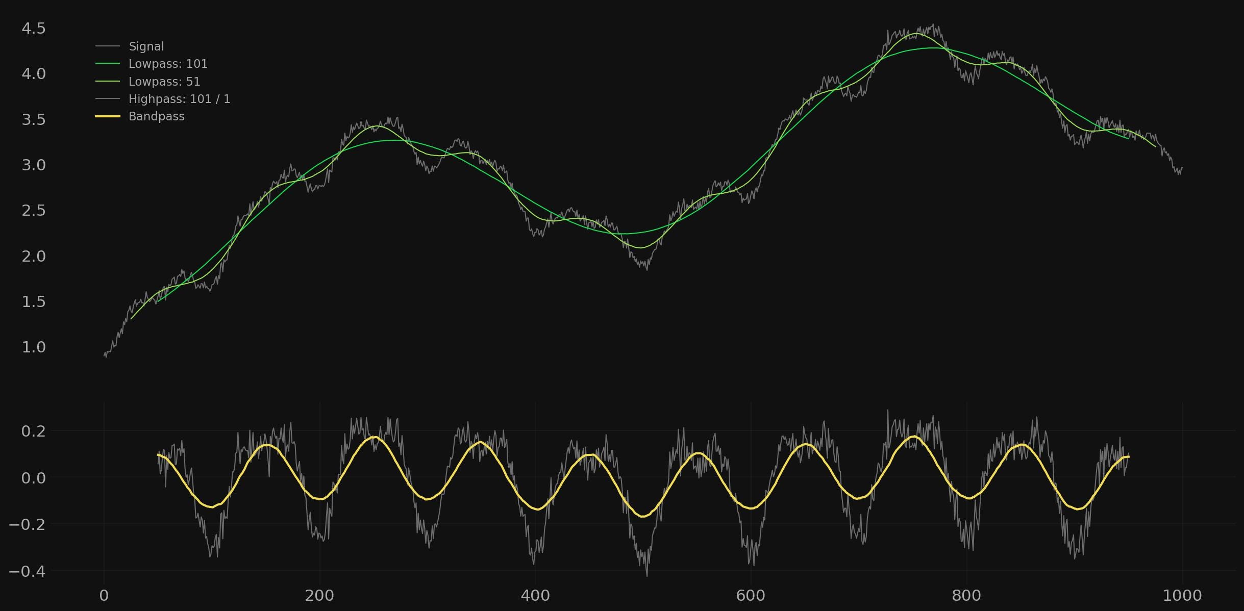
Clearly the obvious difference between these two outputs is that the high pass retains both the noisy part of the signal and the component at a wavelength of 50. The latter can be seen in the slight undulation of the signal between the 100 wavelength component troughs. Both outputs also contain a tiny part of the component at 500 wavelength, an unavoidable feature of using a moving average as a time series filter due to it’s frequency response.
Now you may ask why we can’t just filter the high pass output with a low pass filter to achieve the same result as the bandpass? Well the answer is we can but the additional operation introduces a further filter lag, as demonstrated below.
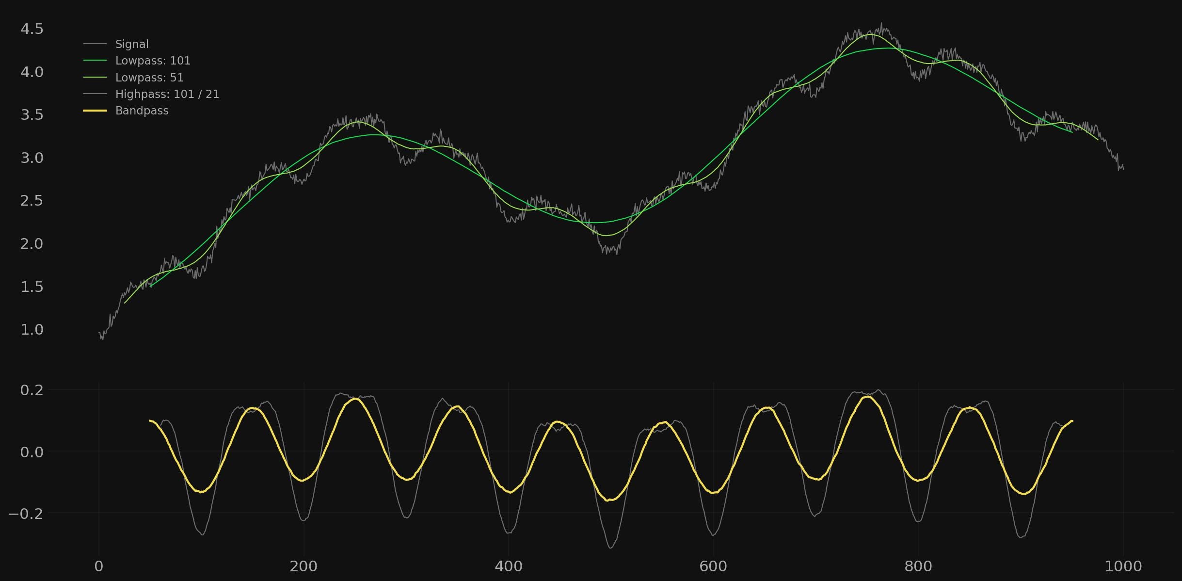
Example 3
In this example we will attempt to extract the component at a wavelength of 50. The amplitude of this component is relatively (and deliberately!) low at 0.1 so we can expect a rather rougher result due to the similar amplitude of the noise component. Indeed the component of 50 wavelength is only slightly visually apparent in the signal.
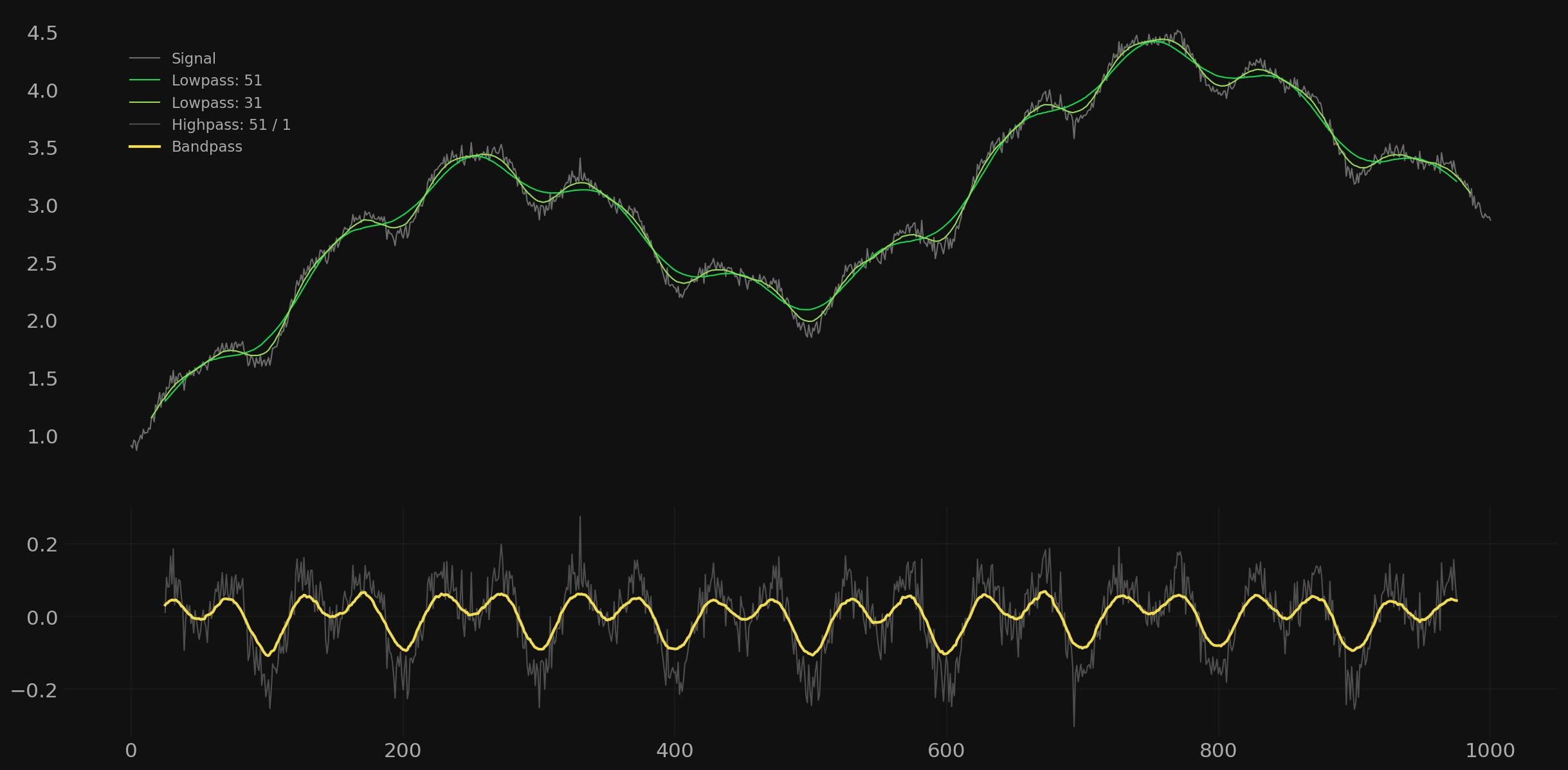
Here the result is somewhat more what we might expect from real markets and amplitude modulated components. The periodic signal of interest is buried deeply in the overall signal and the amplitude is only just above that of the noise. Regardless, a bandpass filter set at 51/31 gives a reasonable result, maintaining the amplitude of around 0.1 and revealing the periodic component. Note how the much higher amplitude component of 100 wavelength is bleeding through. The highpass filter is also shown for comparison with the noise retained in the output.
In Summary
We hope these articles on the humble moving average have been insightful and prompted some of you to look at this staple of technical analysis in a different (and perhaps more correct?) light. All that is required in order to take advantage of the filter characteristics of this indicator is to lag it correctly! New trading strategies and indicators can also be constructed - for example a correctly plotted MACD or RSI. The ubiquitous nature of the incorrectly plotted moving average operation in many indicators implies a ripe ground for experimentation.
The obvious path now is to take this knowledge and apply some moving average style filtering on real markets! Keep an eye out for that article, coming in the next few weeks on Sigma-L.
How do you achieve such smooth output from moving averages?
This series about digital filters is awesome. Thank you! it would be great to have the anticipated upcoming aricles as well :)