

The Moving Average - Done Right
Discover how to supercharge the simple moving average in your analysis

Ubiquity != Accuracy
The above statement is apt to describe the humble moving average and the common use of it as an indicator by technical analysts of financial markets across the world. However, in the vast majority of cases (and certainly by a brief look at some charts on TA twitter), it is being used almost entirely incorrectly! This is also compounded by the fact many indicators employed by chartists to form trading algorithms or signals use moving averages incorrectly in their own composition.
Two such examples are the relative strength index (RSI) and the moving average convergence divergence (MACD).
The Inescapable Digital Filter Lag
To understand why moving averages are being plotted incorrectly in most cases we need to understand what a moving average actually is. It is a data smoother, or, in signal processing parlance, a low pass filter. It is most often utilised to emphasise or ‘uncover’ some kind of price trend, composed of lower frequency components, via the attenuation of higher frequency components. It does this via the mathematical operation of averaging over all data points in a certain window of data points, the length of which is stipulated by the user as the ‘period’ or ‘span’ of the average.
As an example, below is some pseudo code detailing a moving average of span 3, passed over a vector of 5 points, analogous to prices in a financial market over a period of 5 sample points:
data = [2,3,4,8,6] // A 5 point vector of data
ma_span = 3 // The 'span or period' of the moving average

// Step by step calculation:
> 2+3+4 / 3 = 3 // 1st MA data point
> 3+4+8 / 3 = 5 // 2nd MA data point
> 4+8+6 / 3 = 6 // 3rd MA data point
> 8+6+NaN // Not enough points for window!

// Original data and MA vector, incorrectly aligned for time
data = [2,3,4,8,6]
MA =   [3,5,6,-,-]

// Original data and MA vector, correctly aligned for time
data = [2,3,4,8,6]
MA =   [-,3,5,6,-]
The process of averaging via a window, as shown above, results in unavoidable data loss. This is because at the end of the series we simply run out of data points to satisfy the number required for the window of the moving average. In this particular case we lose 2 points at the end of the series. In general terms the equation for the number of points lost due to digital filter lag is simply:
ma_span-1So in the above case where the moving average span is 3, we lose 2 data points.
Because of this loss we must adjust the placement in time on our charts to reflect the loss of data. We are dealing with timeseries for the majority of our charts in financial markets so must adjust accordingly if we wish to judge trend (or other metrics) correctly. A moving average that is plotted at nowtime and not lagged to account for the inherent data loss is attempting to estimate trend via data that reflects that trend incorrectly! This is negligible for a short MA such as the 3MA above but if averages based upon longer spans are employed, as they so often are to smooth data for any use in trend estimation, the larger error inherent renders such lines as useless.
In order to correctly align moving averages with price to account for digital filter lag we must use the following equation to center the average in regard to price and time. This is seen above in the ‘correctly aligned’ data and MA vector:
shift = (ma_span-1)/2Due to the discrete sampling of timeseries in financial markets it is often best to choose an odd span for your moving average when accounting for digital filter lag. This is so the average can be accurately centred using the calculation above. This is not so important for very large moving average calculations.
For example, a moving average of period 11 should be shifted back in time by 5 points. If the moving average was 10, the midpoint would be 4.5, or halfway between two of our discrete sample points.
The fact we have to shift the moving average back in time like this reveals the reason perhaps that many chartists have ignored (knowlingly or not) the correct placement: We lose the moving average at nowtime!
Of course trading decisions are made often on the basis of price interactions at nowtime and a moving average is somewhat compelling for the naive trader/investor. It is though, nonsense, in the majority of cases to infer anything from a non-lagged moving average.
Moving Average = LPF
All is not lost however. What we lose in nowtime clarity we gain back several fold in the ability to utilise the humble moving average as a low pass filter when correctly plotted to account for digital filter lag.
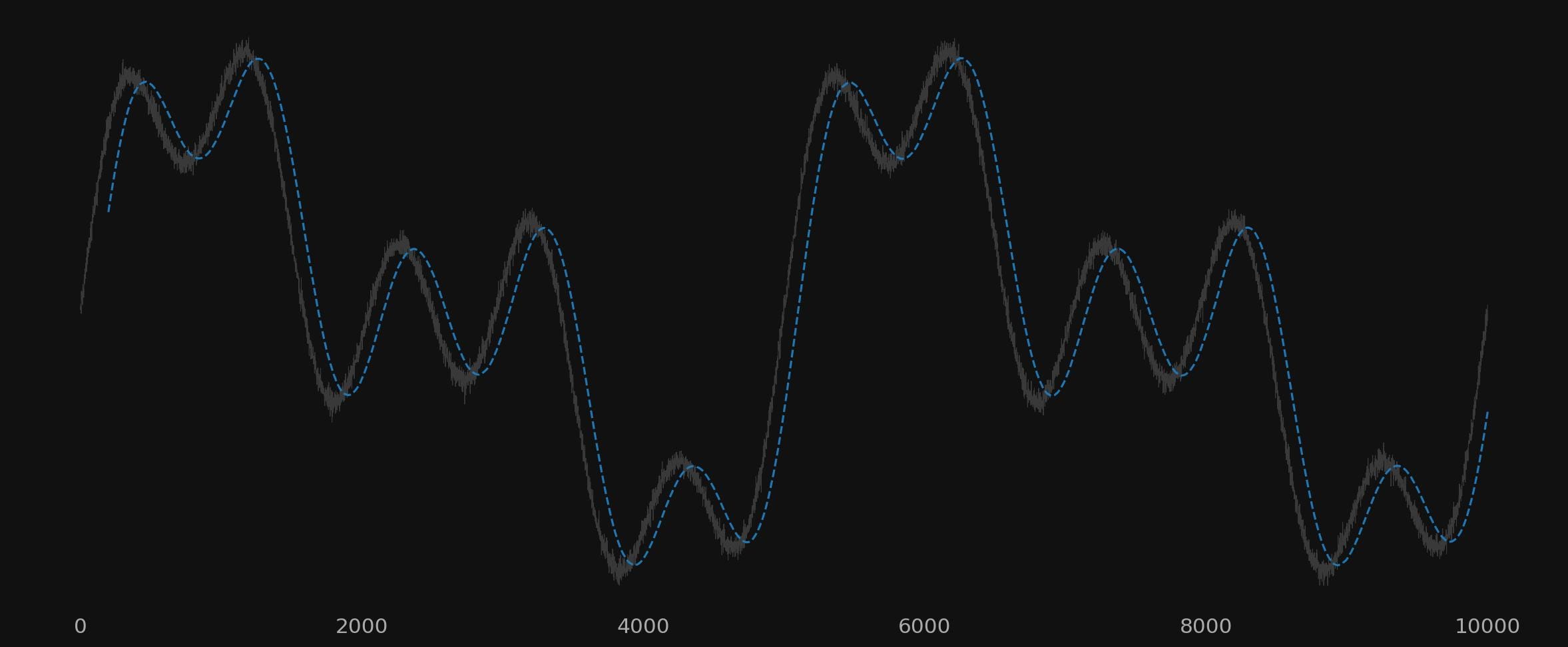
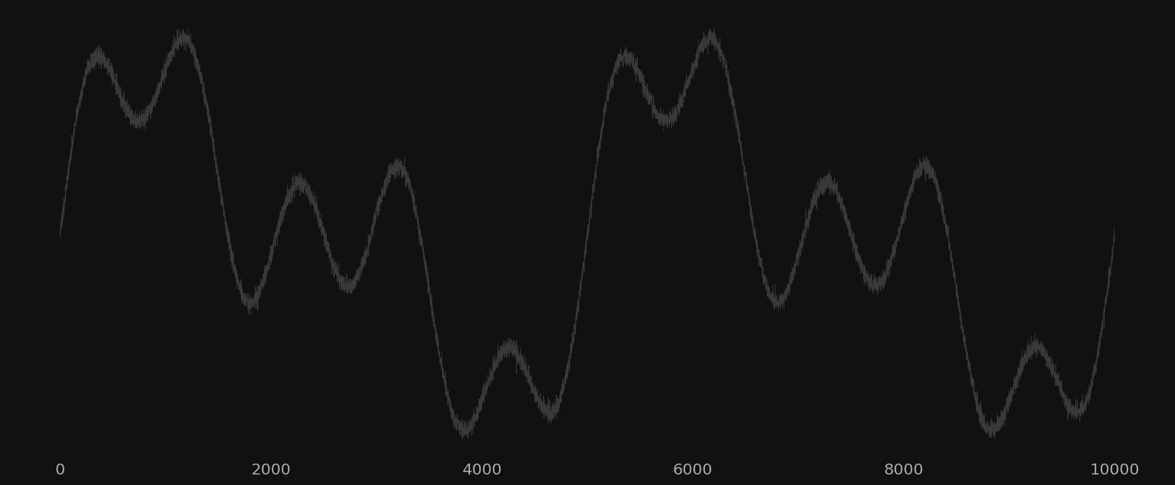
Let’s build a composite timeseries that will consist of simple sine waves and some added gaussian noise before the addition of a moving average to demonstrate a low pass filter. We will see when the average is correctly shifted and span carefully chosen we can begin to utilise the benefits.
A feature of MAs used as low pass filters is the ability to attenuate completely ALL instances of cyclic components in a signal equal to the span of the moving average. This is a wonderful property and leads onto all kinds of possibilities to construct highpass, bandpass and bandstop filters via the humble moving average, available to almost all traders on all platforms.
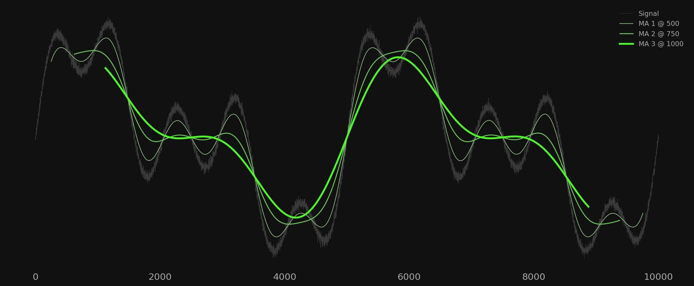
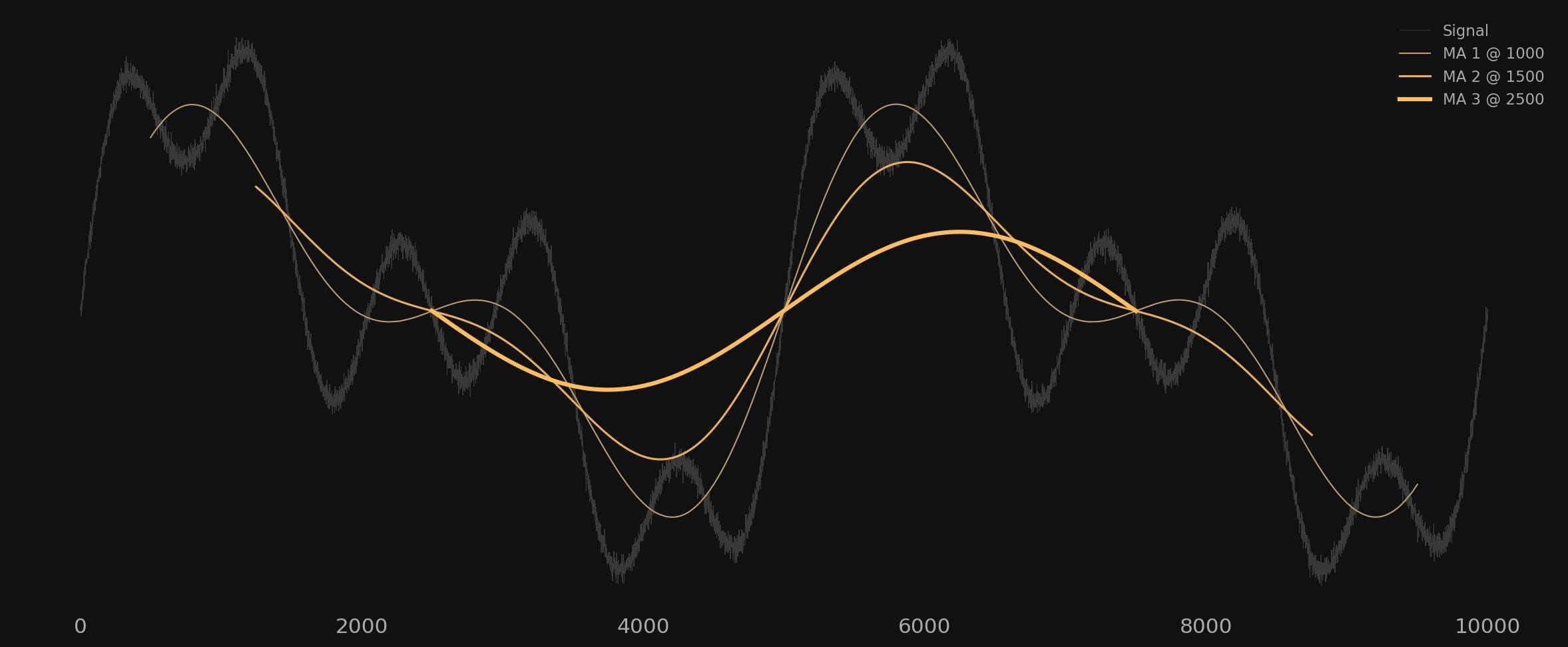
Below, we add 3 moving averages (correctly lagged) that approach the wavelength of the 1000 point component. Note how as the span approaches the wavelength in the signal, it is removed, leaving only the other two components and some tiny residual noise:
Now, let’s try removing the larger wavelength component of 2500, leaving us with a signal consisting only of the component of wavelength 5000.
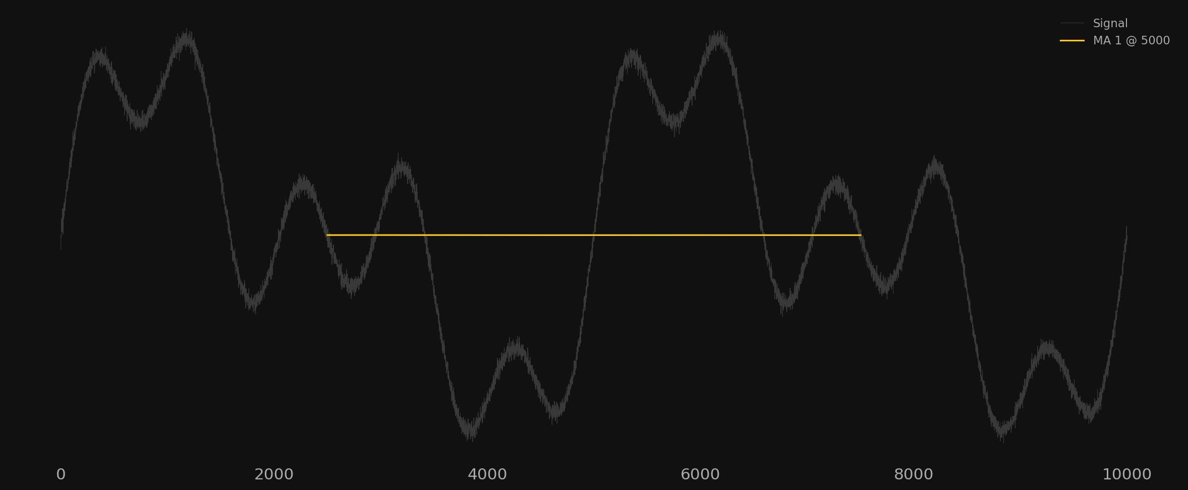
Finally, we attempt to remove the very longest component in this signal with the low pass filter characteristics of the moving average. Since there is no more signal components available after this stage of filtering, we should get a flat line. We use one moving average here with a span of 5000 to match the target wavelength:
In this way we can use the moving average in a useful way to isolate cyclical components of interest in financial markets. It can only be done if the average is correctly lagged though and we pay the price via the necessary shifting of the timeseries.
Solutions to Filter Lag
There are a few solutions available when we need to extrapolate the moving average to nowtime due to the lag inherent in this approach. We will look into one of these in a future article, namely polynomial regression. It is very well suited to approximating such smooth curves and with good benefits at the medium term wavelengths (think 80 day, 20 week, 40 week components in the nominal model).
Flipping the Average
We can also exploit another benefit in using MAs as low pass filters, the ability to ‘flip’ the average and arrive at a highpass filter easily. Hurst called these ‘inverse’ moving averages. It is simply the process of subtracting the low pass filtered timeseries from the original signal. This is where things get really interesting as we can isolate components away from the modulating effects of the very long period trends.
Thanks for the valuable insights David,
Just wanted to check when we use the 5000 span displaced average, the straight line does not appear, instead the moving average is still little curved,
Could you kindly help as to how to make a straight line
Regards
Ak