Underlying Trend: Sigma-L

In this article we look at how to account for the ever present underlying trend in the context of the advanced fld trading strategy explored previously.

Markets Are Never Flat

A simple concept, but one which must be considered for our purposes as Hurstonians, is underlying trend. Named by Hurst as ‘sigma-l’ to simply mean ‘the sum of all cycles’, it is inherent in a system which assumes cycles form an infinite series of increasing period. This underlying trend (which can be thought of as a sum of sinusoidal functions) is never static. It may appear to be flat when shorter cycles form sideways consolidations but this is just a result of a much larger period cycle, relative to the cycle in focus, turning up or down.

Traditional technical analysis has come to love the simple moving average as an indicator of trend, usually set at a arbitrary period of 50, 100 or 200 to smooth higher frequencies. This is a blunt tool and flawed. Firstly by the fact moving averages must be time shifted by the (period/2) to account for the digital filter lag and, secondly, the moving average makes no attempt to decompose the signal, save for it’s low pass characteristics.

In the Cyclitec cycles course Hurst tabulated sigma-l by assessing the phase of each component in question and arriving at an estimation for sigma-l. Below is an example of this in Sentient Trader using the daily phasing of Bitcoin.

Each nominal model component is assessed and given a status of up, down, turning down, turning up. Note the absense of the 9 year and 18 year components because they are not present in the phasing analysis.

In Practice

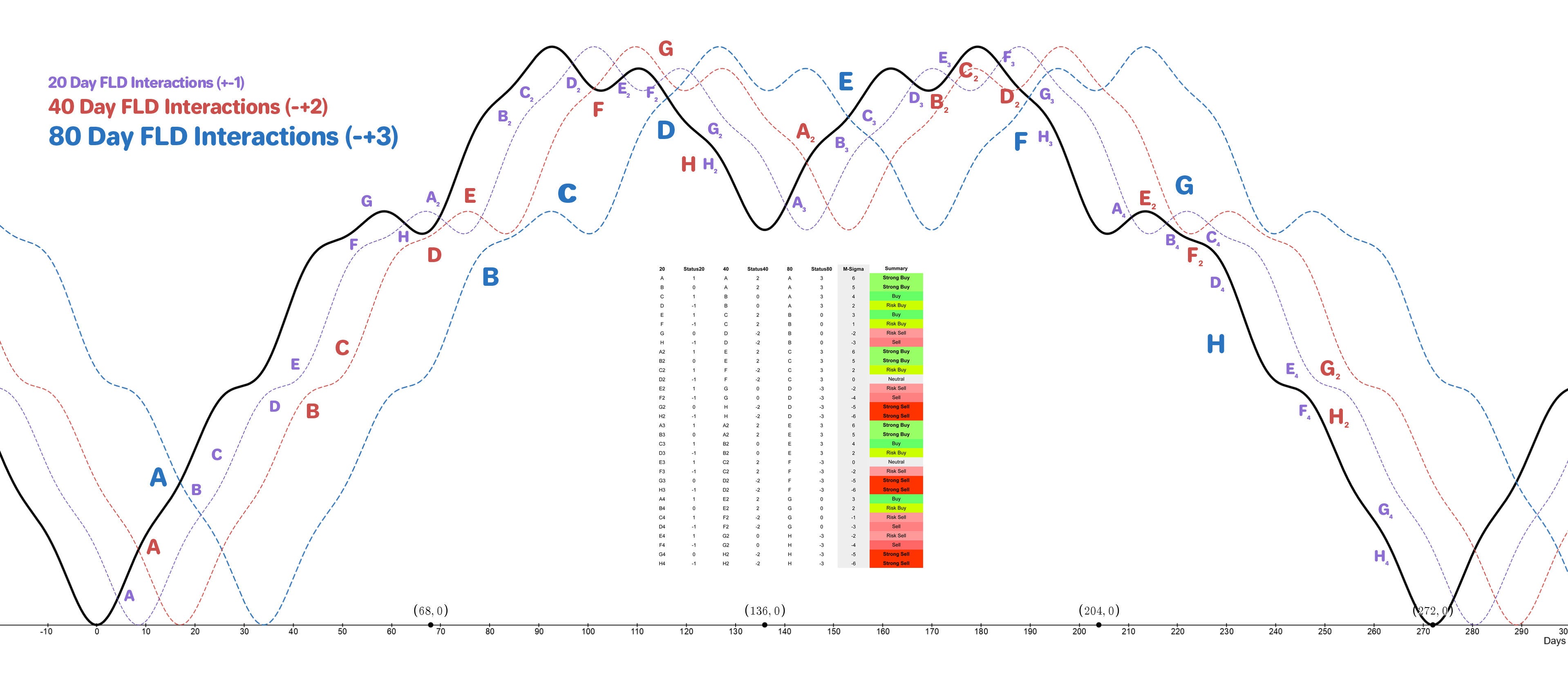
We will take our advanced FLD trading strategy which uses three discrete components of the nominal model and their respective signal cycle FLDs to demonstrate a rudimentary application of sigma-l. In this example we will assign a linear trend to the model and observe the effect on price, interactions and the summary status of ‘M-Sigma’ - our subset of underlying trend only applicable to this 40 week sample.

In real markets the trend is not linear and is the sum of what can be thought of as discrete, sinusoidal functions of increasing wavelength.

The model here assumes a non-existent sigma-l. Put simply, the value of sigma-l is zero. In real markets this is never true, but may be approached if a much longer cycle is either turning up, or turning down.

Trend is Up

Here we assign sigma-l a value of 1 and the dotted line below price is an indicator of it’s function. The effect on the composite price line is obvious with the familiar ‘higher low’ forming at the end of the chart and price skewed upwards.

A bullish (positive) underlying trend modulates the composite summation such that upside targets of already bullish FLD interactions are heavily exceeded. Interactions which were previously expected to just meet downside targets will now be undershot.

Trend is Down

Here we assign sigma-l a value of -1 and the inverse effect of a positive sigma-l is observed. The effect on the composite price line a ‘lower low’ forming at the end of the chart and price skewed downwards.

A bearish (negative) underlying trend modulates the composite summation such that downside targets of already bearish FLD interactions are heavily exceeded. Interactions which were previously expected to just meet upside targets will now be undershot.

We can now look at what effect the addition of this simple linear trend has on our overall summary at each 20 day FLD interaction and the strength of the trade associated with it.

The addition of an underlying trend has an effect on the summary status of each interaction in the series of interactions, informing decisions.

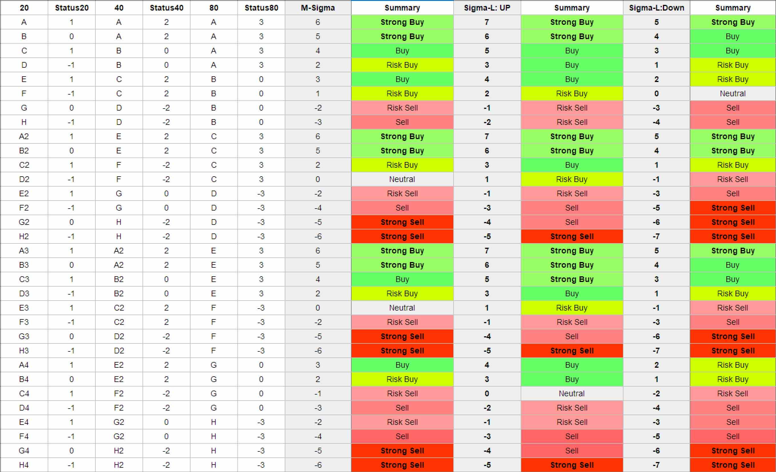
The tabulation above shows the summary of each 20 day FLD interaction in the idealised 40 week period, via the model described previously. M-Sigma shows interaction trade direction and strength when the underlying trend is assumed to be 0, essentially a localised subset of underlying trend.

Subsequent summary columns show the resulting differences when underlying trend is up and down, respectively, as a true reflection of Sigma-L. This more closely resembles real price action in financial markets.

Looking at the summary columns with underlying trend accounted for we can see that in the bullish scenario, those trends previously described as ‘risk buy’ are now standard ‘buys’, some ‘buys’ become ‘strong buys’ and so on. The underlying trend has the effect of amplifying bullish signals and attenuating bearish signals. Of course the inverse is true when the underlying trend is bearish.

---

If you enjoyed this article please consider sharing it with friends and colleagues. Thank you for your continued support and interest in Hurst Cycles.

---

DISCLAIMER: This website/newsletter and the charts/projections contained within it are intended for educational purposes only. Results and projections are hypothetical. We accept no liability for any losses incurred as a result of assertions made due to the information contained within Sigma-L. This report is not intended to instruct investment or purchase of any financial instrument, derivative or asset connected to the information conveyed in the report. Trade and invest at your own risk.