

Free! Tradingview Indicator: 3-Pole Butterworth Bandpass Filter
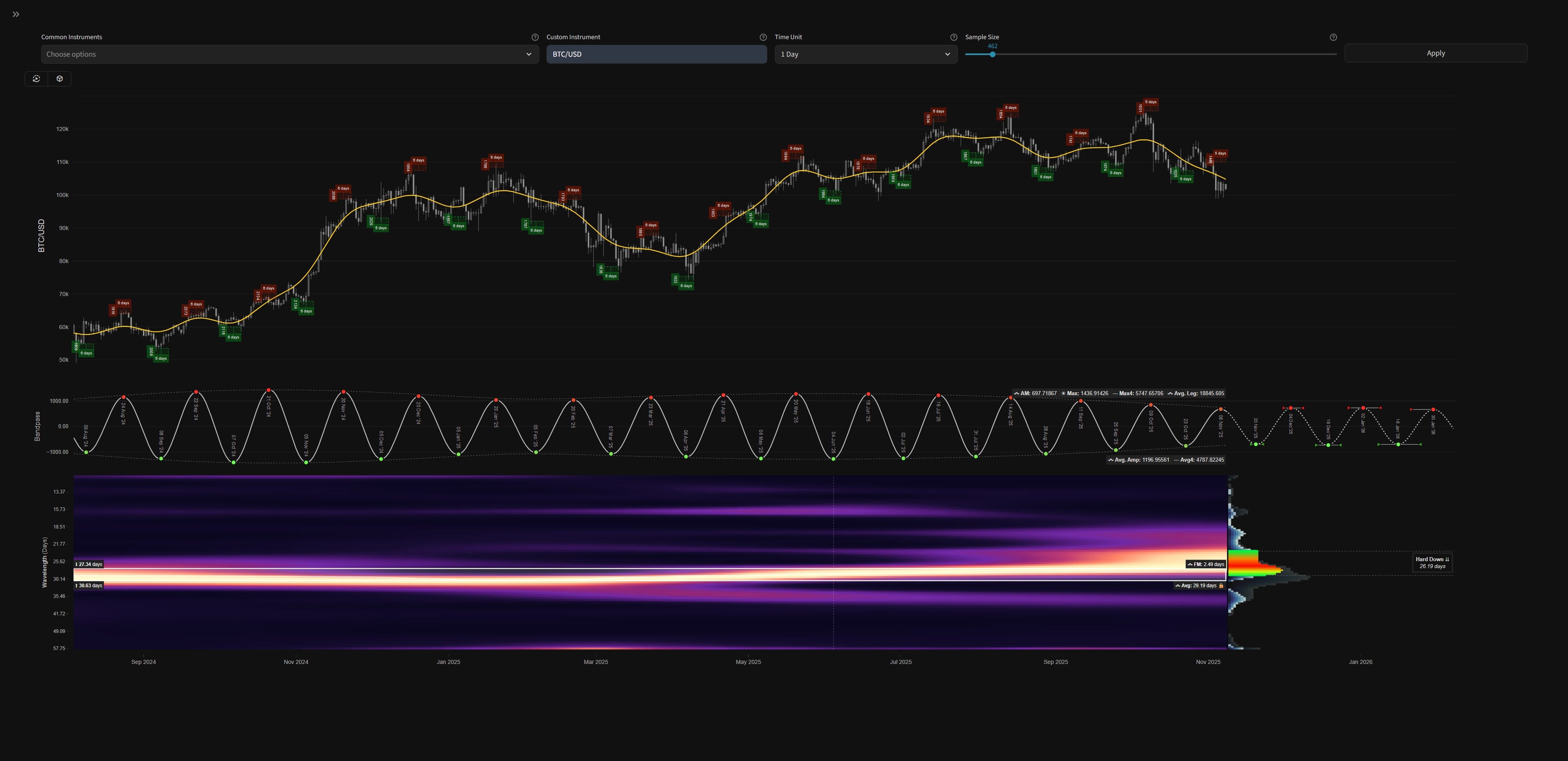
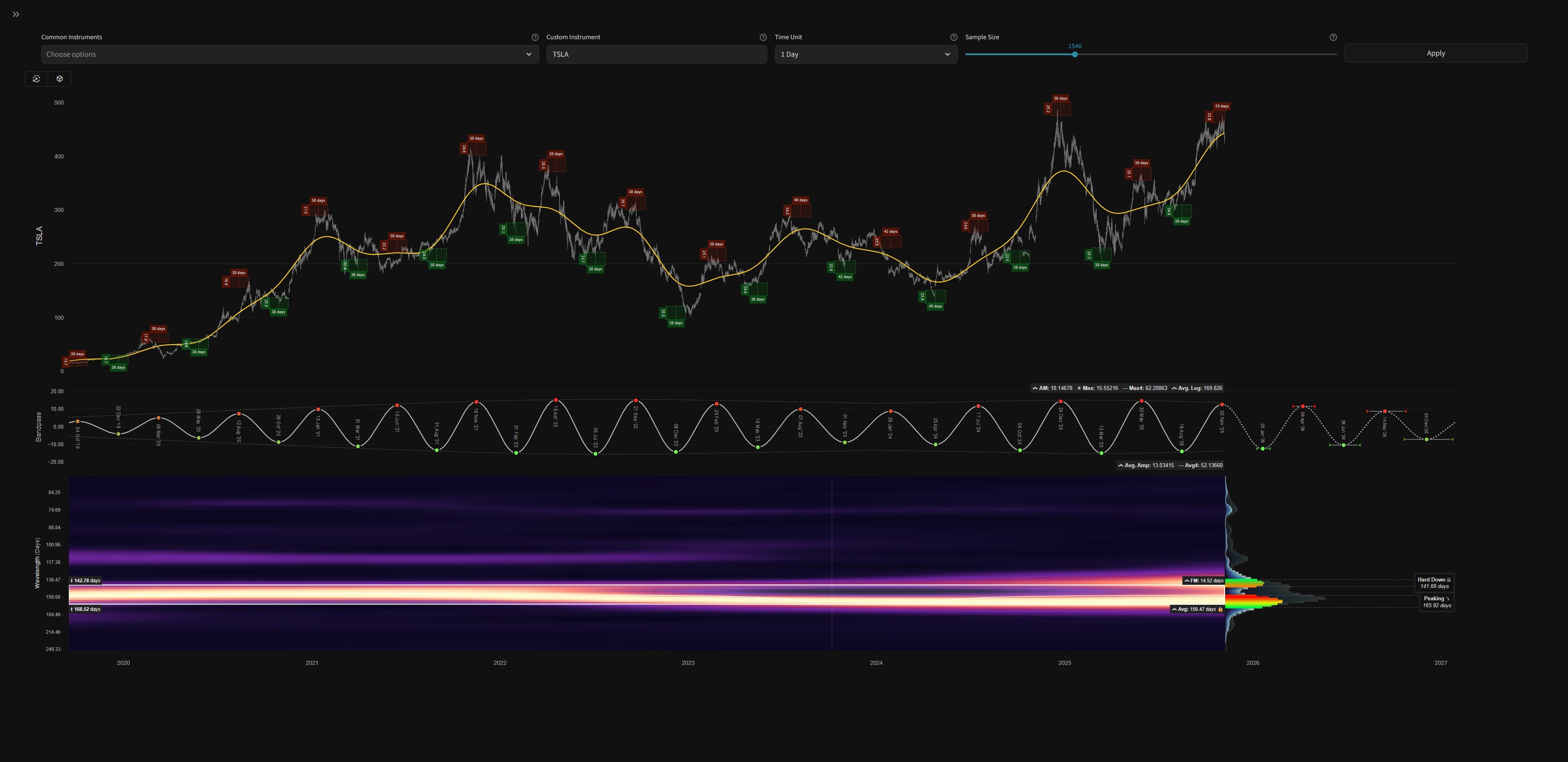
Add a 3 pole Butterworth band pass filter to your price series in Tradingview to help visualise cycles identified by our main time frequency analysis.


Although Tradingview’s pinescript language is, unfortunately, limited for the purpose of performing frequency domain analysis on market data, one can implement time domain filters to a decent degree, given some verbose coding (compared to optimal python/numpy/C and vectorisation).
Below is a fairly simple implementation of a Butterworth bandpass filter (on close prices) for your analysis pleasure. The price series is first detrended prior to filtering using a quadratic (order 2) or cubic (order 3) polynomial fit.
Copy and paste the code into the Tradingview code area to use on your charts, remembering to configure the upper and lower bounds of the filter (the cutoffs) according to your desired cycle target.
It is important to consider when configuring the cutoffs that Tradingview does not interpolate for weekends / holidays as we do in the main time frequency analysis. Therefore cycles identified in the main time frequency analysis will be slightly longer than the cutoffs needed for this Butterworth filter. I recommened experimenting yourself to discover the best parameters for optimal correlation to the time frequency result.

//@version=6
indicator(”Sigma-L BW Sweep”, overlay=false)

// Inputs
low_per = input.int(40, “Low Cutoff Period”, minval=10)
high_per = input.int(80, “High Cutoff Period”, minval=10)
filter_length = input.int(100, “Number of Bars for Filter/Detrend”, minval=20)
detrend_order = input.int(2, “Detrend Order (2 or 3)”, minval=1, maxval=3)
src = input.source(close, “Source”)

// Polynomial Detrend Function (least squares fit for order 2 or 3)
poly_detrend(src_in, len, order) =>
    if len <= order
        src_in
    else
        n = len
        x_mean = (n - 1) / 2.0
        sum_y = 0.0
        sum_z_y = 0.0
        sum_z2_y = 0.0
        sum_z3_y = 0.0
        sum_z2 = 0.0
        sum_z4 = 0.0
        sum_z6 = 0.0
        for i = 0 to n - 1
            xi = float(n - 1 - i)
            zi = xi - x_mean
            yi = src_in[i]
            sum_y += yi
            sum_z_y += zi * yi
            sum_z2_y += zi * zi * yi
            sum_z2 += zi * zi
            sum_z4 += zi * zi * zi * zi
            sum_z3_y += zi * zi * zi * yi
            sum_z6 += zi * zi * zi * zi * zi * zi
        y_mean = sum_y / n
        denom_even = sum_z4 - sum_z2 * sum_z2 / n
        b2 = (sum_z2_y - y_mean * sum_z2) / denom_even
        b0 = y_mean - (sum_z2 / n) * b2
        b1 = 0.0
        b3 = 0.0
        z_current = float(n - 1) - x_mean
        if order == 2
            b1 := sum_z_y / sum_z2
        else
            det = sum_z2 * sum_z6 - sum_z4 * sum_z4
            b1 := (sum_z6 * sum_z_y - sum_z4 * sum_z3_y) / det
            b3 := (sum_z2 * sum_z3_y - sum_z4 * sum_z_y) / det
        trend = b0 + b1 * z_current + b2 * z_current * z_current + b3 * z_current * z_current * z_current
        src_in - trend

// Detrended source
detrended_src = poly_detrend(src, filter_length, detrend_order)

// 3-Pole Butterworth Low-Pass Function
butterLP(src_in, len_in) =>
    cf = 2 * math.tan(math.pi / len_in)
    cf2 = cf * cf
    cf3 = cf2 * cf
    a0 = 8 + 8 * cf + 4 * cf2 + cf3
    a1 = -24 - 8 * cf + 4 * cf2 + 3 * cf3
    a2 = 24 - 8 * cf - 4 * cf2 + 3 * cf3
    a3 = -8 + 8 * cf - 4 * cf2 + cf3
    c = cf3 / a0
    d0 = -a1 / a0
    d1 = -a2 / a0
    d2 = -a3 / a0
    out = 0.0
    out := nz(c * (src_in + src_in[3]) + 3 * c * (src_in[1] + src_in[2]) + d0 * out[1] + d1 * out[2] + d2 * out[3], src_in)
    out

// Band-Pass on detrended series: High-Pass (detrended - LP(high_per)) then LP(low_per)
lp_high = butterLP(detrended_src, high_per)
hp = detrended_src - lp_high
bp_full = butterLP(hp, low_per)

// Plot in indicator window
plot(bp_full, “Butterworth Band-Pass (Detrended)”, color=color.blue, linewidth=2)
hline(0, “Zero Line”, color=color.gray, linestyle=hline.style_dashed)

The Cycle Hunt is On
If, in the course of using this indicator, you discover what you believe to be a metronomic signal (mostly stationary amplitude and frequency!), please let me know so I can run the TFA across it and share it to subscribers. Many pairs of eyes are better than one!
Thanks in advance.
David